OpenCV DNN 패키지를 이용한 Faster RCNN 기반 Object Detection 수행
OpenCV 를 이용하면 DNN API를 따오고, 이를 기반으로 (학습은 못하고) Inference 를 수행할 수 있다고 했다. 지금은 Object Detection을 해볼 것이고, 사용할 모델은 이전까지 이론적으로 학습한 Faster RCNN이다.
기본적으로 OpenCV 는 Tensorflow 에서 Pretrained 된 모델을 로드한다고하였다. 이미지, 모델을 순차적으로 다운받아보자.
이미지는 코랩 상에서 /content/data 밑에 beatles01.jpg 라는 이름으로 만들어줬다. imread()로 읽고, cvtColor() 로 RGB로 바꿔줘서 이미지를 띄워보자!
✅ 이미지 로드
import cv2
import matplotlib.pyplot as plt
%matplotlib inline

img = cv2.imread('./data/beatles01.jpg')
img_rgb = cv2.cvtColor(img, cv2.COLOR_BGR2RGB)

print('image shape:', img.shape)
plt.figure(figsize=(12, 12))
plt.imshow(img_rgb)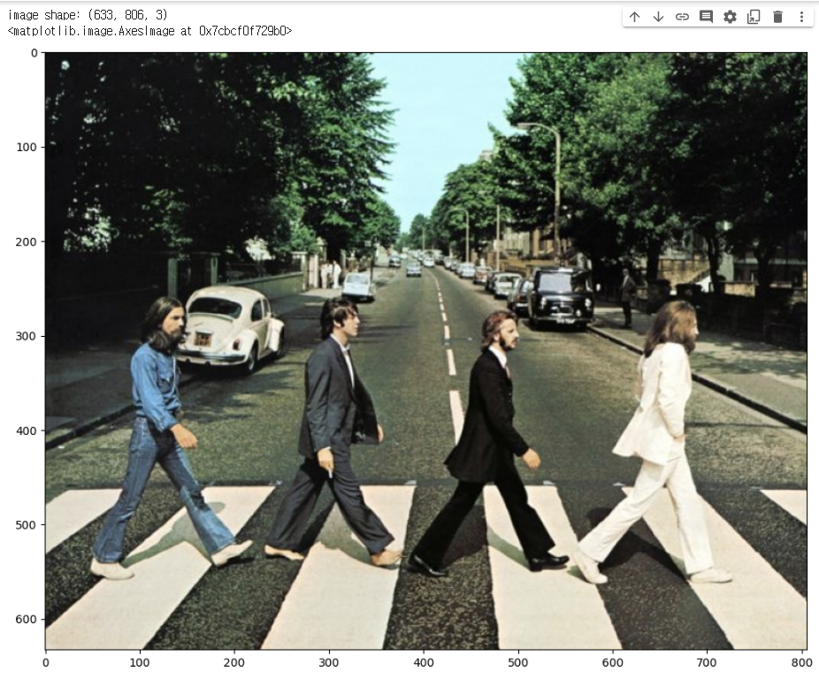
✅ Tensorflow Pretrained Inference 모델, Config 파일 다운로드
mkdir ./pretrained 명령어로 content/pretrained 디렉토리를 만들고 그 밑에 각각 pretrained 모델과 config 파일을 다운로드 받았다. 모델의 경우 .tar 로 압축되어 있는데, !tar 로 압축을 풀고 -C ./pretrained 로 이 밑에 풀 수 있다.
다운로드 URL 은 다음과 같다.
!mkdir ./pretrained
# pretrained 모델
!wget -O ./pretrained/faster_rcnn_resnet50_coco_2018_01_28.tar.gz http://download.tensorflow.org/models/object_detection/faster_rcnn_resnet50_coco_2018_01_28.tar.gz
# config 파일
!wget -O ./pretrained/config_graph.pbtxt https://raw.githubusercontent.com/opencv/opencv_extra/master/testdata/dnn/faster_rcnn_resnet50_coco_2018_01_28.pbtxt

# 압축파일 풀기
!tar -xvf ./pretrained/faster*.tar.gz -C ./pretrained
그러고나서 모델쪽 파일을 확인해보면
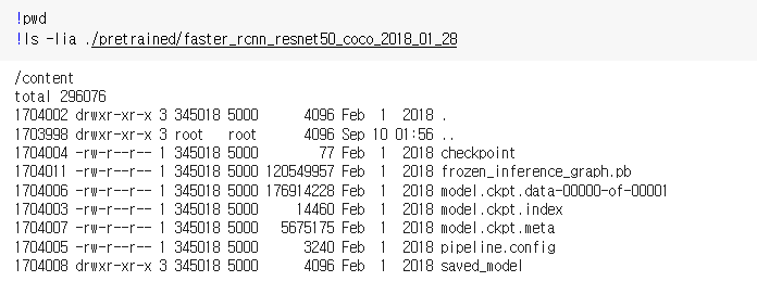
다음과 같이 체크포인트, 메타 정보 등 다양하게 있지만.. 주로 사용하는 파일은 .pb 로 끝나는 모델과 .pbtxt 인 환경파일이다. 여기까지 로딩해주자! 로딩시에는 .readNetFromTensorflow 를 이용하면 된다.
cv_net = cv2.dnn.readNetFromTensorflow('./pretrained/faster_rcnn_resnet50_coco_2018_01_28/frozen_inference_graph.pb','./pretrained/config_graph.pbtxt')✅ 다음으로는 모델, 이미지가 준비되었을 때 또다르게 필요한 클래스명 지정단계이다.
클래스명 지정은 MS COCO데이터 세트에서 숫자와 해당 클래스 이름을 매핑하기 위해 하나의 변수에다 해당 변수들을 딕셔너리로 넣는 것을 말한다. 여기서 헷갈릴 수 있는 점이.. tensorflow 에서 훈련된 모델을 OpenCV에서 돌릴 때 매핑되는 클래스 개수가 조금씩 다르다! 아래 정리된 내용을 확인하자.
- Tensorflow Faster RCNN : 0-90까지
- Tensorflow SSD : 1-91까지
- Tensorflow Mask RCNN : 0-90까지
- Darknet YOLO: 0-79까지
현재는 Faster RCNN에 대한 구현을 할 것이므로 0-90까지 91개로 매핑된 딕셔너리가 필요하다.
# OpenCV Tensorflow Faster-RCNN용 -> 91개
labels_to_names_0 = {0:'person',1:'bicycle',2:'car',3:'motorcycle',4:'airplane',5:'bus',6:'train',7:'truck',8:'boat',9:'traffic light',
                    10:'fire hydrant',11:'street sign',12:'stop sign',13:'parking meter',14:'bench',15:'bird',16:'cat',17:'dog',18:'horse',19:'sheep',
                    20:'cow',21:'elephant',22:'bear',23:'zebra',24:'giraffe',25:'hat',26:'backpack',27:'umbrella',28:'shoe',29:'eye glasses',
                    30:'handbag',31:'tie',32:'suitcase',33:'frisbee',34:'skis',35:'snowboard',36:'sports ball',37:'kite',38:'baseball bat',39:'baseball glove',
                    40:'skateboard',41:'surfboard',42:'tennis racket',43:'bottle',44:'plate',45:'wine glass',46:'cup',47:'fork',48:'knife',49:'spoon',
                    50:'bowl',51:'banana',52:'apple',53:'sandwich',54:'orange',55:'broccoli',56:'carrot',57:'hot dog',58:'pizza',59:'donut',
                    60:'cake',61:'chair',62:'couch',63:'potted plant',64:'bed',65:'mirror',66:'dining table',67:'window',68:'desk',69:'toilet',
                    70:'door',71:'tv',72:'laptop',73:'mouse',74:'remote',75:'keyboard',76:'cell phone',77:'microwave',78:'oven',79:'toaster',
                    80:'sink',81:'refrigerator',82:'blender',83:'book',84:'clock',85:'vase',86:'scissors',87:'teddy bear',88:'hair drier',89:'toothbrush',
                    90:'hair brush'}
✅ Inference
본격적으로 예측을 만드는 코드를 보자! 코드는 2번에 잘라서 보도록 해보자.
# 원본 이미지가 Faster RCNN기반 네트웍으로 입력 시 resize됨.
# 바운딩박스의 예측은 스케일링을 바탕으로 0-1사이에서 이루어짐. 이를 되돌리기 위해 원본 이미지 shape정보 필요
rows = img.shape[0]
cols = img.shape[1]
# cv2의 rectangle()은 인자로 들어온 이미지 배열에 직접 사각형을 업데이트 하므로 그림 표현을 위한 별도의 이미지 배열 생성.
draw_img = img.copy()

# 원본 이미지 배열 BGR을 RGB로 변환하여 배열 입력. Tensorflow Faster RCNN은 마지막 classification layer가 Dense가 아니여서 size를 고정할 필요는 없음.
cv_net.setInput(cv2.dnn.blobFromImage(img, swapRB=True, crop=False))

# Object Detection 수행하여 결과를 cvOut으로 반환
cv_out = cv_net.forward() # -> Inference. 결과가 cv_out 에 저장.
print(cv_out.shape)

# bounding box의 테두리와 caption 글자색 지정
green_color=(0, 255, 0)
red_color=(0, 0, 255)
첫 단계에서 해야할 일은 이미지 행과 열의 shape 저장, 카피, 모델에 입력과 forward 연산이다.
- shape 을 찍어 이미지 행과 열을 저장하는 이유는 Inference 내부적으로 스케일을 통해 바운딩박스의 위치를 나타내기 때문이다. (예를들어 좌상단 좌표 (0.314, 0.215) 이런식으로..) 따라서 해당 좌표를 원래대로 복구하기 위해선 비율이 필요하며, 따라서 rows 와 cols 의 수를 기록해두는 것이다.
- copy() 를 하는 이유는 이미지 자체에 사각형을 그릴 것이므로 원본 이미지는 내버려두기 위해서다. copy 에는 사각형과 캡션을 넣고, 원본 이미지의 경우 모델에 넣고 사각형의 위치만 찾은 후 그 위에 덮어쓰지 않는다.
- 모델에
setInput()을 해준 후forward()연산을 해주면 Object Detection 이 수행되며, 이 결과를 cv_out 에 저장할 수 있다.
# detected 된 object들을 iteration 하면서 정보 추출
for detection in cv_out[0,0,:,:]: # class id, confidence 만큼 루프 (100개)
score = float(detection[2]) # -> 확신정도 /0.98 등등
class_id = int(detection[1]) # -> class id /person
# detected된 object들의 score가 0.5 이상만 추출
if score > 0.5:
# detected된 object들은 scale된 기준으로 예측되었으므로 (0-1) 다시 원본 이미지 비율로 계산 (좌,우는 열비율, 상,하는 행비율 곱!)
left = detection[3] * cols
top = detection[4] * rows
right = detection[5] * cols
bottom = detection[6] * rows
# labels_to_names_seq 딕셔너리로 class_id값을 클래스명으로 변경.
caption = "{}: {:.4f}".format(labels_to_names_0[class_id], score)
print(caption)
#cv2.rectangle()은 인자로 들어온 draw_img에 사각형을 그림. 위치 인자는 반드시 정수형. (이미지, (좌상단), (우하단), corlor, 두께)
cv2.rectangle(draw_img, (int(left), int(top)), (int(right), int(bottom)), color=green_color, thickness=2)
# (이미지, 캡션글자, 좌상단좌표, 폰트,..)
cv2.putText(draw_img, caption, (int(left), int(top - 5)), cv2.FONT_HERSHEY_SIMPLEX, 0.4, red_color, 1)
# 네모상자와 텍스트를 넣고 이미지 컬러를 마지막으로 변환
img_rgb = cv2.cvtColor(draw_img, cv2.COLOR_BGR2RGB)
plt.figure(figsize=(12, 12))
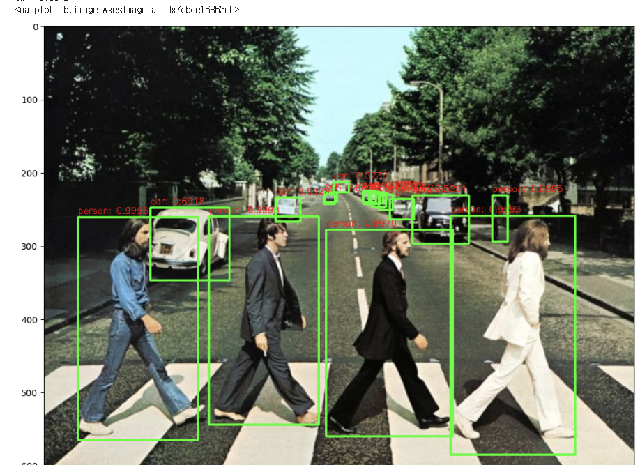
plt.imshow(img_rgb)두번째 단계에서 해야할 일은 반복문을 돌면서 detect 한 오브젝트들의 좌상단 우하단의 좌표를 추출하고, 사각형을 그리고 캡션을 넣는 일이다.
cv_out 에는 어떤 정보가 들어있을까? 우선 cv_out.shape을 찍어보면 1, 1, 100, 7 로 출력이 되고, 이는 [의미없음, 의미없음, object detect 개수, 추가정보] 를 의미한다. 추가정보는 7개의 정보가 하나의 리스트로 들어있으며, [의미없음, class id, class 확신정도, 좌, 상단, 우, 하단좌표] 가 들어가 있다. cv_out 을 찍어보자.
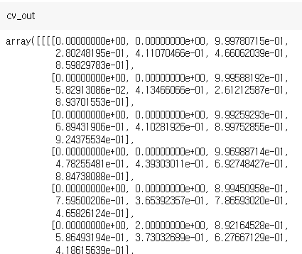
이렇게 detect 된 오브젝트들에 대한 바운딩박스정보가 들어가있다.
따라서 함수 내부적으로도 반복문을 돌며 cv_out[0,0,:,:] 으로 4차원의 첫번째, 3차원의 첫번째, 2차원의 모든 값, 1차원의 모든 값을 가져온다. 100개가 detect 되었으므로 100번 돌 것이다! 인덱스 [2] 를 통해선 score, [1] 을 통해선 class_id 를 가져올 수 있을 것이다.
이때 확신정도가 0.5 이상인 것에 대해서만 좌상단, 우하단의 좌표를 가져오고, 이때는 스케일링 된 위치 X 아까 구해둔 rows or cols 를 곱해주어 좌표를 복구시킨다.
.rectangle() 은 이제 구한 좌표값을 실제 카피한 이미지에 씌울 수 있다. 인자로는 (이미지, (좌상단), (우하단), 색, 두께) 가 들어간다. .putText() 는 이미지에 캡션을 넣을 수 있으며, (이미지, 캡션글, (좌상단), 폰트, 크기, 색, 굵기) 를 인자로 전달한다.
이제 draw_img 사본에는 사각형도 그렸고 텍스트도 넣었으므로 색만 바꿔서 출력하면 된다. 색을 RGB로 바꿀 땐 역시나 .cvtColor() 를 이용한다.
✅ 함수화
방금 본 명령어들을 한데 모아 함수화하자. 인자로 전달할 것은 (모델, 이미지, 임계값, 카피 사용, 프린트사용)이다.
import time
# 모델, 이미지, threshold
def get_detected_img(cv_net, img_array, score_threshold, use_copied_array=True, is_print=True):

    rows = img_array.shape[0]
    cols = img_array.shape[1]

    draw_img = None
    if use_copied_array:
        draw_img = img_array.copy()
    else:
        draw_img = img_array

    cv_net.setInput(cv2.dnn.blobFromImage(img_array, swapRB=True, crop=False))

    start = time.time()
    cv_out = cv_net.forward()

    green_color=(0, 255, 0)
    red_color=(0, 0, 255)

    # detected 된 object들을 iteration 하면서 정보 추출
    for detection in cv_out[0,0,:,:]:
        score = float(detection[2])
        class_id = int(detection[1])
        # detected된 object들의 score가 함수 인자로 들어온 score_threshold 이상만 추출
        if score > score_threshold:
            # detected된 object들은 scale된 기준으로 예측되었으므로 다시 원본 이미지 비율로 계산
            left = detection[3] * cols
            top = detection[4] * rows
            right = detection[5] * cols
            bottom = detection[6] * rows
            # labels_to_names 딕셔너리로 class_id값을 클래스명으로 변경. opencv에서는 class_id + 1로 매핑해야함.
            caption = "{}: {:.4f}".format(labels_to_names_0[class_id], score)
            print(caption)
            #cv2.rectangle()은 인자로 들어온 draw_img에 사각형을 그림. 위치 인자는 반드시 정수형.
            cv2.rectangle(draw_img, (int(left), int(top)), (int(right), int(bottom)), color=green_color, thickness=3)
            cv2.putText(draw_img, caption, (int(left), int(top - 5)), cv2.FONT_HERSHEY_SIMPLEX, 0.5, red_color, 1)
    if is_print:
        print('Detection 수행시간:',round(time.time() - start, 2),"초")

    return draw_img
✅ 함수활용
이제 짜놓은 get_detected_img 를 통해 다른 사진에 대해서도 테스트 할 수 있다. 나는 곰돌이 사진이 포함된 이미지를 object Detection 해봤다. 참고로 핸드폰 사진을 찍어서 업로드할 시 픽셀이 너무 많아 예측속도가 느려질 수 있는데, 이때는 imutils.resize() 메서드를 이용해서 resolution 을 조금 낮춰주도록 하자. 나의 경우 width=800 으로 주면 예측속도 7초 정도에 해당 detection 이 가능했다.
import imutils
img_gom = cv2.imread('/content/data/곰돌이.jpg')
resized_gom = imutils.resize(img_gom, width=800)

# tensorflow inference 모델 로딩
cv_net = cv2.dnn.readNetFromTensorflow('./pretrained/faster_rcnn_resnet50_coco_2018_01_28/frozen_inference_graph.pb',
                                     './pretrained/config_graph.pbtxt')
# Object Detetion 수행 후 시각화
draw_img = get_detected_img(cv_net, resized_gom, score_threshold=0.95, use_copied_array=True, is_print=True)

img_rgb = cv2.cvtColor(draw_img, cv2.COLOR_BGR2RGB)

plt.figure(figsize=(9, 9))
plt.imshow(img_rgb)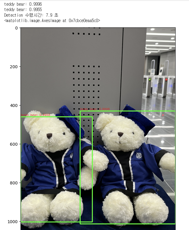
예측시간이 픽셀과 강하게 연결되어 있다는 것을 알았고, 실제 사진을 바꿔가며 넣어보면서 score_threshold 가 얼마나 민감하게 동작하는지도 알았다. 내 경험상 사진의 사이즈를 작게할수록 bounding box도 크게크게 잡아서, 사진에 잡고싶은 물체가 그렇게 많지 않은 경우에는 resize 로 사진을 작게하고 잡아내는 것이 오히려 더 깔끔했다. 사진의 크기가 커지면 threshold 를 아무리 높여도 올바르게 detect 하는 것이 더 어려워질수도 있었다 ㅜㅜ.
