[Interest] The multivariate normal distribution

(본 포스팅은 2023-1 성균관대 수학교육과 확률통계학1의 수업 중 다변수 정규분포를 다룬 강의를 정리한 것입니다. 강의 내용과 필기한 피피티의 저작권 모두 이에 있습니다.)

The multivariate normal distribution

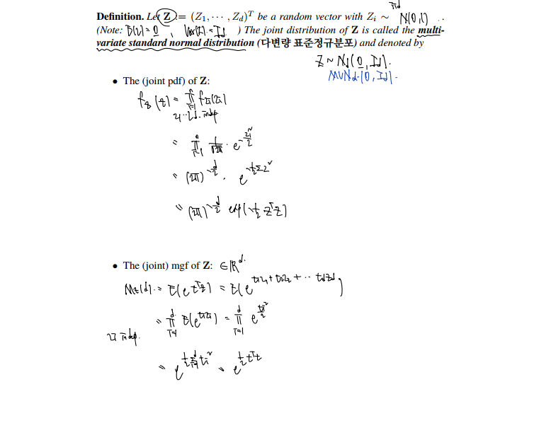
Z = Z1, ..., Zd 가 Z ~ N(0,1) 을 따르는 random vector 라 할 때, joint distribution of Z is called the multi variate standard normal distribution 이라 한다.

The pdf of Z, mfg if Z.

Fact (Spectral Decomposition Theore, 스펙트럼 분해정리)

• Let A be d x d matrix
• and A is a real, symmetric matrix
• Then d x d orthogonal matrix and diagonal matrix 가 있을 때, A는 다음과 같이 정의가 가능하다.

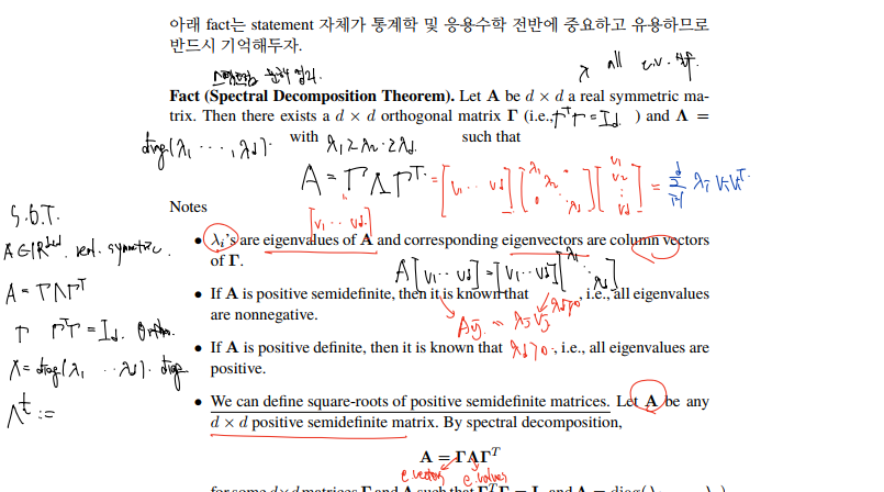
• 람다i는 A의 eigenvalues고, 감마의 column vectors 는 A의 eigenvectors 가 되므로 이는 분해정리라 불린다.
• 람다 >= 0 일 때 A는 positive semidefinite, 람다 > 0 이면 A는 positive definite 이다.
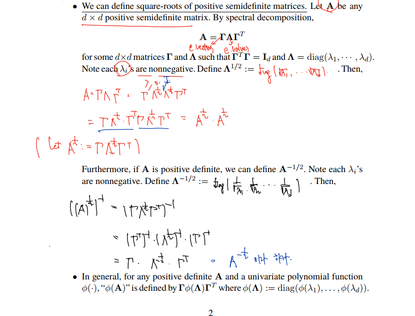
• 이어지는 내용으로, A^1/2 와 A^-1/2 를 정의하는 것이 가능하다.

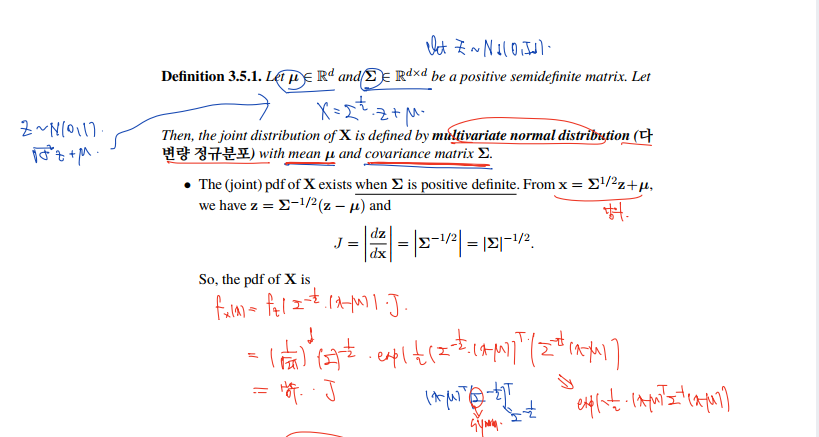
Multivariate normal distribution

Contour plot of f(x)

• 람다^1/2x 만큼 늘리고
• 감마x만큼 회전하고 (Orthogonal 이므로 회전)
• 뮤에 대해 대칭이동해서 contour plot 을 그린다.

Properties of the multivariate normal distribution

1) MVN을 선형변환해도 정규분포이다.

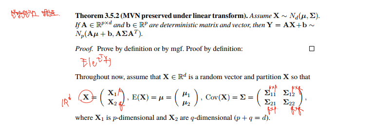
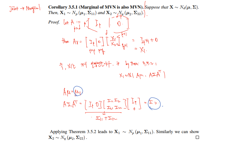
2) Marginal of MVN is also MVN
전체 MVN 의 X 를 X1, X2로 나눠도 이들 각각이 MVN임을 증명할 수 있다.

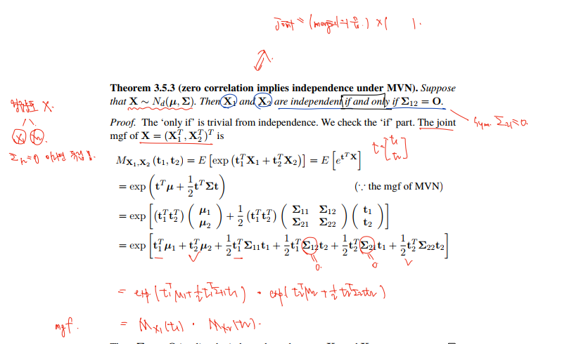
3) Zero correlation 은 MVN 하에서 독립을 의미한다. (공분산행렬12=0 을 이용, joint mfg가 marginal product of mgf 로 계산 가능하다.)

4) MVN의 Conditional distribution 또한 MVN이다. -> 이 증명은 PRML 할 때 했었다!

5) 카이제곱 분포와의 관계

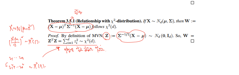
• N(0, I) 를 따르는 MVN Z에서 출발.
• 구하려는 값은 Z^TZ이다.
• 따라서 각 요소를 제곱한 시그마(z^2) 와 같고,
• 이전에 X ~N(평균, 분산) 을 따를 때 제곱의 합의 분포는 카이제곱(n)이라 한 적 있다.
• 이를 적용하여 시그마(z^2) d까지 더함으로 카이제곱(d)를 따르는 것이 증명된다.