1.모듈 정의
모델 학습과 검증 함수를 정의한다.
코드가 길지만, 세세하게 설명을 적어 놓았다. 그러니 겁먹지 말고
코드를 차근차근 보도록 하자.
우선 makedirs를 통해 module이라는 패키지를 만든다.
이 코드는 여러번 실행하지 말자.
이미 만들어진 패키지를 또 만들려고 하면 오류가 나기 때문이다.
import os
os.makedirs('module', exist_ok=True) #module이라는 패키지를 만든 것이다.
그런 다음, 평가하는 코드, train 하는 코드, 최종적으로 학습을 시키는 코드 등을 정의한다.
맨 위의
%%writefile module/train.py
는 module/train.py에 덮어씌우겠다는 의미이다.
%%writefile module/train.py

#이 셀을 실행을 하면 위의 파일에 내용을 쓰라는 이야기이다. 이 점을 반드시 기억할 것!
import torch
import time


#다중분류 문제에 대해 평가하는 코드.
def test_multi_classification(dataloader, model, loss_fn, device="cpu") -> tuple:
    """
    다중 분류 검증/평가 함수

    [parameter]
        dataloader: DataLoader - 검증할 대상 데이터로더
        model: 검증할 모델
        loss_fn: 모델 추정값과 정답의 차이를 계산할 loss 함수.
        device: str - 연산을 처리할 장치. default-"cpu", gpu-"cuda"
    [return]
        tuple: (loss, accuracy)
    """
    model.eval() # 모델을 평가모드로 변환
    size = len(dataloader.dataset) # 전체 데이터수---전체 데이터수를 구하기 위해 dataloader 중에서도 dataset을 구한다.
    num_batches = len(dataloader)  #  step 수

    test_loss, test_accuracy = 0., 0.

    with torch.no_grad():
        for X, y in dataloader:
            X, y = X.to(device), y.to(device)
            pred = model(X) #모델에게 추론을 시키는 부분의 코드이다.
            test_loss += loss_fn(pred, y).item()
            # 정확도 계산
            pred_label = torch.argmax(pred, axis=-1) #label을 뽑아내는 과정이 틀리다.
            test_accuracy += torch.sum(pred_label == y).item()

        test_loss /= num_batches
        test_accuracy /= size  #전체 개수로 나눈다.
    return test_loss, test_accuracy  #결국 test_loss, test_accuracy를 return 한다.


#이중분류에 대해 평가하는 코드. 이렇게 분류하는 이유는 함수도 다르고, 프로세스도 다르기 때문이다.
def test_binary_classification(dataloader, model, loss_fn, device="cpu") -> tuple:
    """
    이진 분류 검증/평가 함수

    [parameter]
        dataloader: DataLoader - 검증할 대상 데이터로더
        model: 검증할 모델
        loss_fn: 모델 추정값과 정답의 차이를 계산할 loss 함수.
        device: str - 연산을 처리할 장치. default-"cpu", gpu-"cuda"
    [return]
        tuple: (loss, accuracy)
    """
    model.eval() # 모델을 평가모드로 변환
    size = len(dataloader.dataset)
    num_batches = len(dataloader)

    test_loss, test_accuracy = 0., 0.

    with torch.no_grad():
        for X, y in dataloader:
            X, y = X.to(device), y.to(device)
            pred = model(X)
            test_loss += loss_fn(pred, y).item()
            ## 정확도 계산
            pred_label = (pred >= 0.5).type(torch.int32) #정확도가 일정 기준 이상이면,이를 pred_label에 추가.
            test_accuracy += (pred_label == y).sum().item()

        test_loss /= num_batches
        test_accuracy /= size   #전체 개수로 나눈다.
    return test_loss, test_accuracy


#train 해주는 코드를 작성했다.
def train(dataloader, model, loss_fn, optimizer, device="cpu", mode:"binary or multi"='binary'):
    """
    모델을 1 epoch 학습시키는 함수

    [parameter]
        dataloader: DataLoader - 학습데이터셋을 제공하는 DataLoader
        model - 학습대상 모델
        loss_fn: 모델 추정값과 정답의 차이를 계산할 loss 함수.
        optimizer - 최적화 함수
        device: str - 연산을 처리할 장치. default-"cpu", gpu-"cuda"
        mode: str - 분류 종류. binary 또는 multi
    [return]
        tuple: 학습후 계산한 Train set에 대한  train_loss, train_accuracy
    """
    model.train()
    size = len(dataloader.dataset) #총 데이터수

    for batch, (X, y) in enumerate(dataloader): #batch의 수와 x,y도 출력을 시도!
        X, y = X.to(device), y.to(device)
        pred = model(X) #모델 학습

        loss = loss_fn(pred, y) #loss 구하기

        optimizer.zero_grad() #gradient 초기화
        loss.backward()
        optimizer.step()
        #이를 통해 한 step의 학습이 끝났다.

    if mode == 'binary': #모드에 따라서 train 관련값이 어떻게 반영이 될 것인지에 대한 놈이다.
        train_loss, train_accuracy = test_binary_classification(dataloader, model, loss_fn, device)
    else:
        train_loss, train_accuracy = test_multi_classification(dataloader, model, loss_fn, device)
    return train_loss, train_accuracy


#최종적으로 학습을 시킨다. 학습을 하고, 검증을 하는 것 2가지를 같이 한다.
def fit(train_loader, val_loader, model, loss_fn, optimizer, epochs,
        save_best_model=True, save_model_path=None, early_stopping=True, patience=10, device='cpu',  mode:"binary or multi"='binary',
    lr_scheduler=None):
    """
    모델을 학습시키는 함수

    [parameter]
        train_loader (Dataloader): Train dataloader
        test_loader (Dataloader): validation dataloader
        model (Module): 학습시킬 모델
        loss_fn (_Loss): Loss function
        optimizer (Optimizer): Optimizer
        epochs (int): epoch수
        save_best_model (bool, optional): 학습도중 성능개선시 모델 저장 여부. Defaults to True.
        save_model_path (str, optional): save_best_model=True일 때 모델저장할 파일 경로. Defaults to None.
        early_stopping (bool, optional): 조기 종료 여부. Defaults to True.
        patience (int, optional): 조기종료 True일 때 종료전에 성능이 개선될지 몇 epoch까지 기다릴지 epoch수. Defaults to 10.
        device (str, optional): device. Defaults to 'cpu'.
        mode(str, optinal): 분류 종류. "binary(default) or multi
    [return]
        tuple: 에폭 별 성능 리스트. (train_loss_list, train_accuracy_list, validation_loss_list, validataion_accuracy_list)
        lr_scheduler:Learning Rate 스케쥴러 객체. default: None
    """

    train_loss_list = []
    train_accuracy_list = []
    val_loss_list = []
    val_accuracy_list = []

    #이런 거는 상황에 맞게 알맞게 사용하면 된다.
    if save_best_model:
        best_score_save = torch.inf

    ############################
    # early stopping
    #############################
    if early_stopping:
        trigger_count = 0
        best_score_es = torch.inf

    # 모델 device로 옮기기
    model = model.to(device)
    s = time.time()
    for epoch in range(epochs):

        train_loss, train_accuracy = train(train_loader, model, loss_fn, optimizer, device=device, mode=mode)
        #train이라는 함수를 호출하면, train_loss와 train_accuracy를 return 할 것이다.
       #이 과정을 통해 train 과정이 끝이 난다.(한 epoch의 train이 끝이 난다.)

        # 검증 - test_xxxx_classsification() 함수를 호출한다. mode가 무엇인가에 따라 코드의 동작 방식이 달라진다.
        if mode == "binary":
            val_loss, val_accuracy = test_binary_classification(val_loader, model, loss_fn, device=device)
        else:
            val_loss, val_accuracy = test_multi_classification(val_loader, model, loss_fn, device=device)

        ####LR Scheduler에게 lr 변경요청
        if lr_scheduler:
            lr_scheduler.step()

        #한 에폭의 검증 결과를 각 list에 추가한다.
        train_loss_list.append(train_loss)
        train_accuracy_list.append(train_accuracy)
        val_loss_list.append(val_loss)
        val_accuracy_list.append(val_accuracy)

        #로그 출력. 현재 epoch, train loss, train accucracy 등을 세세히 출력한다.
        print(f"Epoch[{epoch+1}/{epochs}] - Train loss: {train_loss:.5f} Train Accucracy: {train_accuracy:.5f} || Validation Loss: {val_loss:.5f} Validation Accuracy: {val_accuracy:.5f}")
        print('='*100)

        # 모델 저장
        if save_best_model:
            if val_loss < best_score_save:
                torch.save(model, save_model_path)
                print(f"저장: {epoch+1} - 이전 : {best_score_save}, 현재: {val_loss}")
                best_score_save = val_loss

        # early stopping 처리 (early stopping이 true인지 false인지 따져 보는 것이다.)
        if early_stopping: #true라면 스코어를 갱신하고 trigger를 0으로 설정한다.
            if val_loss < best_score_es:
                best_score_es = val_loss
                trigger_count = 0

            else:
                trigger_count += 1
                if patience == trigger_count:
                    print(f"Early stopping: Epoch - {epoch}")
                    break

    e = time.time()
    print(e-s, "초")
    return train_loss_list, train_accuracy_list, val_loss_list, val_accuracy_list


#이 코드는 복습 시간에 정말 세세하게 코드 리뷰를 하도록 하자.
2.dataset 생성 함수 제공 모듈
dataset을 생성 함수 제공 모듈도 따로 정의를 하는 편이 더 좋다.
%%writefile module/data.py

#이번엔 data.py라는 이름을 가진 파일에 저장을 하자.
from torchvision import datasets, transforms
from torch.utils.data import DataLoader

def load_mnist_dataset(root_path, batch_size, is_train=True):
    """
    mnist dataset dataloader 제공 함수
    [parameter]
        root_path: str|Path - 데이터파일 저장 디렉토리
        batch_size: int
        is_train: bool = True - True: Train dataset, False - Test dataset
    [return]
        DataLoader
    """
    transform = transforms.Compose([
        transforms.ToTensor()
    ])
    #dataset과 dataloader를 정의한다.
    dataset = datasets.MNIST(root=root_path, train=is_train, download=True, transform=transform)
    dataloader = DataLoader(dataset, batch_size=batch_size, shuffle=is_train)  # shuffle: train이면 True, test면 False 할 것이므로 is_train을 넣음.

    return dataloader #dataloader를 return 하면 결과적으로는 dataset도 같이 포함하는 거야. 위에 코드 보면 알겠지?

def load_fashion_mnist_dataset(root_path, batch_size, is_train=True):
    """
    fashion mnist dataset dataloader 제공 함수
    [parameter]
        root_path: str|Path - 데이터파일 저장 디렉토리
        batch_size: int
        is_train: bool = True - True: Train dataset, False - Test dataset
    [return]
        DataLoader
    """
    transform = transforms.Compose([
        transforms.ToTensor()
    ])
    dataset = datasets.FashionMNIST(root=root_path, train=is_train, download=True, transform=transform)
    dataloader = DataLoader(dataset, batch_size=batch_size, shuffle=is_train)  # shuffle: train이면 True, test면 False 할 것이므로 is_train을 넣음.

    return dataloader
이렇게 dataloader를 정의하고, 실제로 data들을 불러와보자.
3.import
본격적으로 시작하기 앞서, 라이브러리들을 import 하는 것도 잊지 말자.
import torch
import torch.nn as nn

import torchinfo


from module import train, data
import os
import matplotlib.pyplot as plt

device = "cuda" if torch.cuda.is_available() else "cpu" #device에 대한 if문.
device(print로 cpu가 나온다.)
4.하이퍼 파라미터, 변수 정의
이렇게 미리 정의하는 이유는 나중에 변수를 변경하고 싶을 때, 이 코드 부분에 와서 변경하면 더 쉽고 빠르기 때문이다.
LR = 0.001
N_EPOCH = 10
BATCH_SIZE = 200


#DATASET, MODEL 을 저장할 ROOT 디렉토리 경로
DATASET_ROOT_PATH = 'datasets'
MODEL_SAVE_ROOT_PATH = 'models'

#이런 식으로 자주 쓰이거나, 나중에 튜닝의 대상이 되는 변수들은 한 곳에 모아서 정의를 하는 것이 좋다.
#이 팁은 다른 개발을 할 때도 요긴하게 쓰인다.
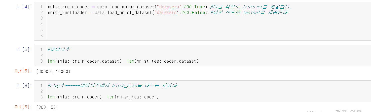
5.data준비-mnist 데이터 로딩
train_loader = data.load_mnist_dataset(DATASET_ROOT_PATH,BATCH_SIZE,True)
test_loader = data.load_mnist_dataset(DATASET_ROOT_PATH,BATCH_SIZE,False)
6.모델의 크기 변경에 따른 성능변화
먼저, 작은 모델을 만들어보자.
#자, 일단 작은 크기의 모델을 한번 적용시켜보자.

class SmallSizeModel(nn.Module):

    def __init__(self):
        super().__init__()
        self.output = nn.Linear(784,10) #in:feature의 수. (1*28*28), out: class 개수------바로 출력하는 것이다.


    def forward(self,X):
        out = nn.Flatten()(X)
        out =self.output(out)
        return out
그러면, summary를 보도록 하자.
small_model = SmallSizeModel()
torchinfo.summary(small_model,(BATCH_SIZE,1,28,28))

#summary를 보면 알겠지만, 뭔가가 많이 있지는 않다.
결과를 한번 볼까?
==========================================================================================
Layer (type:depth-idx)                   Output Shape              Param #
==========================================================================================
SmallSizeModel                           [200, 10]                 --
├─Linear: 1-1                            [200, 10]                 7,850
==========================================================================================
Total params: 7,850
Trainable params: 7,850
Non-trainable params: 0
Total mult-adds (M): 1.57
==========================================================================================
Input size (MB): 0.63
Forward/backward pass size (MB): 0.02
Params size (MB): 0.03
Estimated Total Size (MB): 0.67
==========================================================================================
그런 다음, loss 함수와 optimizer를 정의한다.
#loss

loss_fn = nn.CrossEntropyLoss()

#optimizer
optimizer = torch.optim.Adam(small_model.parameters(),lr=LR)
최종적으로, 앞서 정의했던 train.fit을 통해 한번에 학습을 시킨다.
#train -> module.fit()
#train.fit() 으로 한번에 학습이 된다.
train_loss_list, train_acc_list, valid_loss_list, valid_acc_list = \
train.fit(train_loader,test_loader,small_model,loss_fn,optimizer,N_EPOCH,save_best_model=True,
          save_model_path=os.path.join(MODEL_SAVE_ROOT_PATH,"small_model.pth"),device=device,mode="multi")
아래는 결과를 나타낸 것이다.
Epoch[1/10] - Train loss: 0.44705 Train Accucracy: 0.88607 || Validation Loss: 0.42795 Validation Accuracy: 0.89460
====================================================================================================
저장: 1 - 이전 : inf, 현재: 0.4279545383155346
Epoch[2/10] - Train loss: 0.35787 Train Accucracy: 0.90365 || Validation Loss: 0.34362 Validation Accuracy: 0.90870
====================================================================================================
저장: 2 - 이전 : 0.4279545383155346, 현재: 0.34361504584550856
Epoch[3/10] - Train loss: 0.32298 Train Accucracy: 0.91173 || Validation Loss: 0.31384 Validation Accuracy: 0.91350
====================================================================================================
저장: 3 - 이전 : 0.34361504584550856, 현재: 0.3138397286832333
Epoch[4/10] - Train loss: 0.30486 Train Accucracy: 0.91592 || Validation Loss: 0.29697 Validation Accuracy: 0.91750
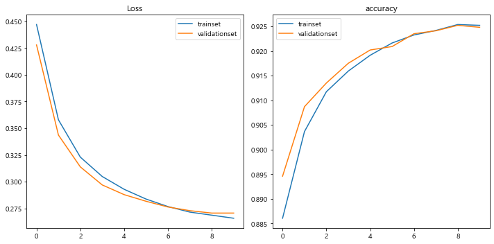
====================================================================================================7.그래프로 그리기
loss와 accuracy의 변동추이를 그래프로 나타낸다.
plt.figure(figsize=(10,5))
plt.subplot(1,2,1)
plt.plot(train_loss_list,label="trainset")
plt.plot(valid_loss_list,label="validationset")
plt.title("Loss")
plt.legend()


plt.subplot(1,2,2)
plt.plot(train_acc_list,label="trainset")
plt.plot(valid_acc_list,label="validationset")
plt.title("accuracy")
plt.legend()

plt.tight_layout()
plt.show()


#뭐 어쨌든 loss는 줄어들고 accuracy는 줄어든 것을 볼 수 있다. 근데, epoch을 더 돌려야 하는 것은 자명하다.
#근본적인 이유는 모델의 크기가 작아서 학습 능력이 떨어지는 것이다.
8.bigsize 모델
앞서서 smallsize모델을 만들었으니, 이번에는 bigsize 모델을 만들어보자.
#자, 이번에는 bigsize 모델을 한번 만들어보자.
## nn.Sequential을 통해 중간 과정을 더 간단하게 만들 수 있다.

class BigSizeModel(nn.Module):
    def __init__(self):
        super().__init__()
        self.b1 = nn.Sequential(nn.Linear(784,2048),nn.ReLU()) #nn.ReLU에 넣겠다는 의미이다.
        self.b2 = nn.Sequential(nn.Linear(2048,1024),nn.ReLU())
        self.b3 = nn.Sequential(nn.Linear(1024,512),nn.ReLU())
        self.b4 = nn.Sequential(nn.Linear(512,256),nn.ReLU())
        self.b5 = nn.Sequential(nn.Linear(256,128),nn.ReLU())
        self.b6 = nn.Sequential(nn.Linear(128,64),nn.ReLU())

        #최종 결과 10개를 출력하게 될 것이다.
        self.output = nn.Linear(64,10)

    def forward(self,X):

        #이런 식으로 각 블록을 통과한다. 이 코드가 없으면, 블록이 정의만 되지 블록을 통과하지는 못한다.
        X = nn.Flatten()(X) #객체를 생성하고 코드를 실행 시키는 것을 항상 잊지 마라!
        out =self.b1(X)
        out =self.b2(out)
        out =self.b3(out)
        out =self.b4(out)
        out =self.b5(out)
        out =self.b6(out)
        return self.output(out)
모델을 정의했으면, 실제로 객체를 생성해보자.
big_model = BigSizeModel()

torchinfo.summary(big_model,(BATCH_SIZE,1,28,28))
결과는 다음과 같이 나온다.
==========================================================================================
Layer (type:depth-idx)                   Output Shape              Param #
==========================================================================================
BigSizeModel                             [200, 10]                 --
├─Sequential: 1-1                        [200, 2048]               --
│    └─Linear: 2-1                       [200, 2048]               1,607,680
│    └─ReLU: 2-2                         [200, 2048]               --
├─Sequential: 1-2                        [200, 1024]               --
│    └─Linear: 2-3                       [200, 1024]               2,098,176
│    └─ReLU: 2-4                         [200, 1024]               --
├─Sequential: 1-3                        [200, 512]                --
│    └─Linear: 2-5                       [200, 512]                524,800
│    └─ReLU: 2-6                         [200, 512]                --
├─Sequential: 1-4                        [200, 256]                --
│    └─Linear: 2-7                       [200, 256]                131,328
│    └─ReLU: 2-8                         [200, 256]                --
├─Sequential: 1-5                        [200, 128]                --
│    └─Linear: 2-9                       [200, 128]                32,896
│    └─ReLU: 2-10                        [200, 128]                --
├─Sequential: 1-6                        [200, 64]                 --
│    └─Linear: 2-11                      [200, 64]                 8,256
│    └─ReLU: 2-12                        [200, 64]                 --
├─Linear: 1-7                            [200, 10]                 650
==========================================================================================
Total params: 4,403,786
Trainable params: 4,403,786
Non-trainable params: 0
Total mult-adds (M): 880.76
==========================================================================================
Input size (MB): 0.63
Forward/backward pass size (MB): 6.47
Params size (MB): 17.62
Estimated Total Size (MB): 24.71
==========================================================================================
summary를 보고 있으면, 가면 갈수록 output shape가 줄어드는 것을 볼 수 있다.
그런 다음에, loss_fn, optimizer 등을 새롭게 적어준다.
#loss_fn, optimizer 등을 새로 적어주는 것이 좋다.

loss_fn = nn.CrossEntropyLoss()
optimizer = torch.optim.Adam(big_model.parameters())
그런 다음, small size model에서 했던 것처럼 학습을 한다.
#학습----위의 것과 다른 것은 파일 등의 이름이다.
#시간이 조금 걸린다.
#train -> module.fit()
#train.fit() 으로 한번에 학습이 된다.
train_loss_list2, train_acc_list2, valid_loss_list2, valid_acc_list2 = \
train.fit(train_loader,test_loader,big_model,loss_fn,optimizer,N_EPOCH,save_best_model=True,
          save_model_path=os.path.join(MODEL_SAVE_ROOT_PATH,"big2_model.pth"),device=device,mode="multi")
아래는 그 결과의 일부이다.
Epoch[1/10] - Train loss: 0.11916 Train Accucracy: 0.96580 || Validation Loss: 0.12917 Validation Accuracy: 0.96260
====================================================================================================
저장: 1 - 이전 : inf, 현재: 0.12916784353554248
Epoch[2/10] - Train loss: 0.07325 Train Accucracy: 0.97773 || Validation Loss: 0.10755 Validation Accuracy: 0.96990
====================================================================================================(중략)
Epoch[10/10] - Train loss: 0.01603 Train Accucracy: 0.99523 || Validation Loss: 0.09420 Validation Accuracy: 0.97880
====================================================================================================근데 사이즈가 크다 보니, 시간이 오래 걸리는 문제가 있다.
small size는 200초 가량이었는데, 이거는 550초 가량이다.
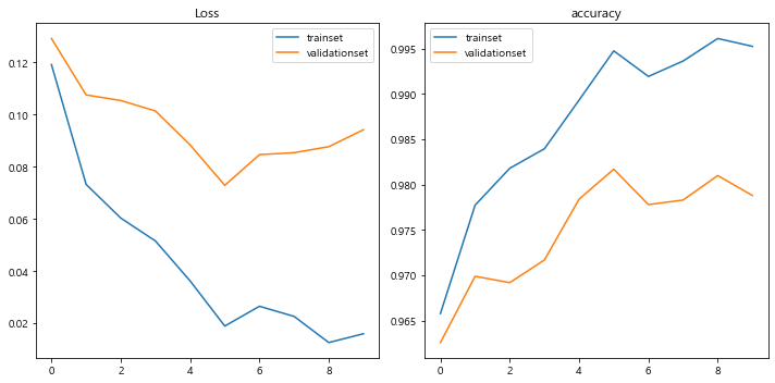
9.bigsize model의 결과 출력
이렇게 loss들을 출력하는 데에 성공했으면, 그래프를 통해 loss의 양이
어떻게 되어가는지를 잘 파악하는 것이 좋다.
plt.figure(figsize=(10,5))
plt.subplot(1,2,1)
plt.plot(train_loss_list2,label="trainset")
plt.plot(valid_loss_list2,label="validationset")
plt.title("Loss")
plt.legend()


plt.subplot(1,2,2)
plt.plot(train_acc_list2,label="trainset")
plt.plot(valid_acc_list2,label="validationset")
plt.title("accuracy")
plt.legend()

plt.tight_layout()
plt.show()


#사이즈가 커지니까.... 여윽시 성능이 더 좋아지는 것 갑다잉.
아무래도 사이즈를 더 크게 하니까 성능이 더 좋아지는 느낌이 든다.
10.dropout 예제
뭐 간단하다. dropout을 각 단계에 적용한다.
dropout은 nn.Dropout 객체를 사용한다.
dropout_rate는 0.2~0.5사이이다.
아래는 DropoutModel의 코드이다.
#Model은 Model인데, dropout을 적용시키는 model이다.

class DropoutModel(nn.Module):


    def __init__(self,drop_rate=0.5):
        super().__init__()
        self.b1 = nn.Sequential(nn.Linear(784,256), nn.ReLU(),nn.Dropout(p=drop_rate)) #보통 거의 모든 단계에 dropout을 적용한다.
        self.b2 = nn.Sequential(nn.Linear(256,256), nn.ReLU(),nn.Dropout(p=drop_rate))
        self.b3 = nn.Sequential(nn.Linear(256,128), nn.ReLU(),nn.Dropout(p=drop_rate))
        self.b4 = nn.Sequential(nn.Linear(128,128), nn.ReLU(),nn.Dropout(p=drop_rate))
        self.output = nn.Sequential(nn.Linear(128,10),nn.Dropout(p=drop_rate))

    def forward(self,X):
        out = nn.Flatten()(X)
        out = self.b1(out)
        out = self.b2(out)
        out = self.b3(out)
        out = self.b4(out)
        out = self.output(out)

        return out
그런 다음, 모델 객체를 정의한 다음, summary를 통해 정보를 요약한다.
d_model = DropoutModel().to(device)
torchinfo.summary(d_model,(BATCH_SIZE,1,28,28)) #summary를 통해 정보를 출력한다.

#relu 뿐만 아니라, dropout도 파라미터가 없다. 학습을 하는 것이 없기 때문이다.
아래는 summary 정보이다.
==========================================================================================
Layer (type:depth-idx)                   Output Shape              Param #
==========================================================================================
DropoutModel                             [200, 10]                 --
├─Sequential: 1-1                        [200, 256]                --
│    └─Linear: 2-1                       [200, 256]                200,960
│    └─ReLU: 2-2                         [200, 256]                --
│    └─Dropout: 2-3                      [200, 256]                --
├─Sequential: 1-2                        [200, 256]                --
│    └─Linear: 2-4                       [200, 256]                65,792
│    └─ReLU: 2-5                         [200, 256]                --
│    └─Dropout: 2-6                      [200, 256]                --
├─Sequential: 1-3                        [200, 128]                --
│    └─Linear: 2-7                       [200, 128]                32,896
│    └─ReLU: 2-8                         [200, 128]                --
│    └─Dropout: 2-9                      [200, 128]                --
├─Sequential: 1-4                        [200, 128]                --
│    └─Linear: 2-10                      [200, 128]                16,512
│    └─ReLU: 2-11                        [200, 128]                --
│    └─Dropout: 2-12                     [200, 128]                --
├─Sequential: 1-5                        [200, 10]                 --
│    └─Linear: 2-13                      [200, 10]                 1,290
│    └─Dropout: 2-14                     [200, 10]                 --
==========================================================================================
Total params: 317,450
Trainable params: 317,450
Non-trainable params: 0
Total mult-adds (M): 63.49
==========================================================================================
Input size (MB): 0.63
Forward/backward pass size (MB): 1.24
Params size (MB): 1.27
Estimated Total Size (MB): 3.14
==========================================================================================
그럼 다음 학습을 시키기 위한 정의 과정을 거친다.
#학습을 시키기 위한 정의 과정

loss_fn = nn.CrossEntropyLoss()
optimizer = torch.optim.Adam(d_model.parameters(),lr=LR)


result = train.fit(train_loader,test_loader,d_model,loss_fn,optimizer,N_EPOCH,save_best_model=False,early_stopping=False,
                  device=device,mode="multi")
결과이다.
Epoch[1/10] - Train loss: 0.29768 Train Accucracy: 0.93248 || Validation Loss: 0.28599 Validation Accuracy: 0.93300
====================================================================================================(중략)
Epoch[10/10] - Train loss: 0.08628 Train Accucracy: 0.97927 || Validation Loss: 0.11161 Validation Accuracy: 0.97150
====================================================================================================
179.66910767555237 초
결과를 보면, train과 valid간의 loss차이가 얼마 나지 않는 것을 목격할 수 있다.
이를 통해 우리는 dropout을 통해 valid와 train 간의 loss 차이를 극복할 수 있음을 알 수 있다.
11.Batch Normalization
Batch Normalization에 대해서도 모델을 만들어보자.
#Linear ->BatchNorm -> Activation(-> Dropout)
#batch normalization에 대한 모델을 만들어보자.

class BNModel(nn.Module):

    def __init__(self):
        super().__init__()
        self.b1 = nn.Sequential(nn.Linear(784,256),nn.BatchNorm1d(256),nn.ReLU()) #속성의 개수를 BatchNorm1d에 넣으면된다.
        #Linear 자체가 1차원이기 때문에, 함수도 1d를 넣으면 된다.
        self.b2 = nn.Sequential(nn.Linear(256,128),nn.BatchNorm1d(128),nn.ReLU())
        self.b3 = nn.Sequential(nn.Linear(128,64),nn.BatchNorm1d(64),nn.ReLU())
        self.output = nn.Linear(64,10)


    def forward(self,X):
        out = nn.Flatten()(X)
        out = self.b1(out)
        out = self.b2(out)
        out = self.b3(out)
        out = self.output(out)
        return out
이제, 모델을 생성하자.
#모델 생성

bn_model = BNModel().to(device)
torchinfo.summary(bn_model,(BATCH_SIZE,1,28,28))
모델 생성에 대한 결과이다.
==========================================================================================
Layer (type:depth-idx)                   Output Shape              Param #
==========================================================================================
BNModel                                  [200, 10]                 --
├─Sequential: 1-1                        [200, 256]                --
│    └─Linear: 2-1                       [200, 256]                200,960
│    └─BatchNorm1d: 2-2                  [200, 256]                512
│    └─ReLU: 2-3                         [200, 256]                --
├─Sequential: 1-2                        [200, 128]                --
│    └─Linear: 2-4                       [200, 128]                32,896
│    └─BatchNorm1d: 2-5                  [200, 128]                256
│    └─ReLU: 2-6                         [200, 128]                --
├─Sequential: 1-3                        [200, 64]                 --
│    └─Linear: 2-7                       [200, 64]                 8,256
│    └─BatchNorm1d: 2-8                  [200, 64]                 128
│    └─ReLU: 2-9                         [200, 64]                 --
├─Linear: 1-4                            [200, 10]                 650
==========================================================================================
Total params: 243,658
Trainable params: 243,658
Non-trainable params: 0
Total mult-adds (M): 48.73
==========================================================================================
Input size (MB): 0.63
Forward/backward pass size (MB): 1.45
Params size (MB): 0.97
Estimated Total Size (MB): 3.05
==========================================================================================
결과를 보면, 각 단계에 따라 output의 크기가 줄어듬을 알 수 있다.
나머지 설정을 해주고, 출력을 통해 결과를 알아내어 보자.
#train
#loss
LR=0.001
loss_fn = nn.CrossEntropyLoss()
optimizer = torch.optim.Adam(bn_model.parameters(),lr=LR)

result_bn = train.fit(train_loader,test_loader,bn_model,loss_fn,optimizer,N_EPOCH,
                      save_best_model=False,early_stopping=False,device=device,mode='multi')
다음은 결과이다.
Epoch[1/10] - Train loss: 0.09036 Train Accucracy: 0.97698 || Validation Loss: 0.11132 Validation Accuracy: 0.96910
====================================================================================================
Epoch[2/10] - Train loss: 0.04656 Train Accucracy: 0.98708 || Validation Loss: 0.07588 Validation Accuracy: 0.97860
====================================================================================================
Epoch[3/10] - Train loss: 0.03109 Train Accucracy: 0.99148 || Validation Loss: 0.07732 Validation Accuracy: 0.97520
====================================================================================================
Epoch[4/10] - Train loss: 0.02708 Train Accucracy: 0.99228 || Validation Loss: 0.06780 Validation Accuracy: 0.97860
====================================================================================================
Epoch[5/10] - Train loss: 0.02121 Train Accucracy: 0.99370 || Validation Loss: 0.06961 Validation Accuracy: 0.97800
====================================================================================================
Epoch[6/10] - Train loss: 0.01245 Train Accucracy: 0.99673 || Validation Loss: 0.06260 Validation Accuracy: 0.98020
====================================================================================================
Epoch[7/10] - Train loss: 0.01088 Train Accucracy: 0.99695 || Validation Loss: 0.06588 Validation Accuracy: 0.97990
====================================================================================================
Epoch[8/10] - Train loss: 0.01000 Train Accucracy: 0.99683 || Validation Loss: 0.06663 Validation Accuracy: 0.98100
====================================================================================================
Epoch[9/10] - Train loss: 0.00834 Train Accucracy: 0.99760 || Validation Loss: 0.06831 Validation Accuracy: 0.98110
====================================================================================================
Epoch[10/10] - Train loss: 0.00692 Train Accucracy: 0.99793 || Validation Loss: 0.07395 Validation Accuracy: 0.98020
====================================================================================================
176.39130353927612 초
결과를 보면, 1번째 epoch보다 10번째 epoch이 더 accuracy가 늘고,
loss는 준 것을 알 수 있다.
12.Learning rate decay
파이토치는 torch.optim 모듈에서 다양한 Learning rate 알고리즘을 제공한다.
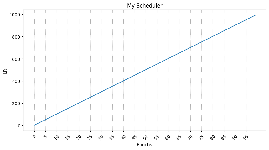
자세한 내용은 다음과 같다.
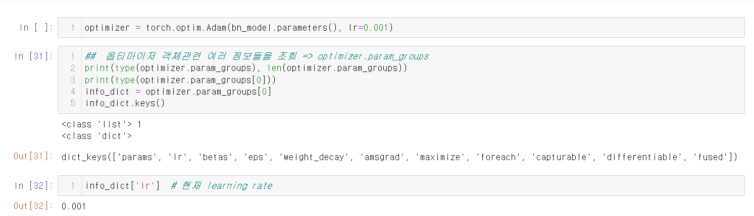
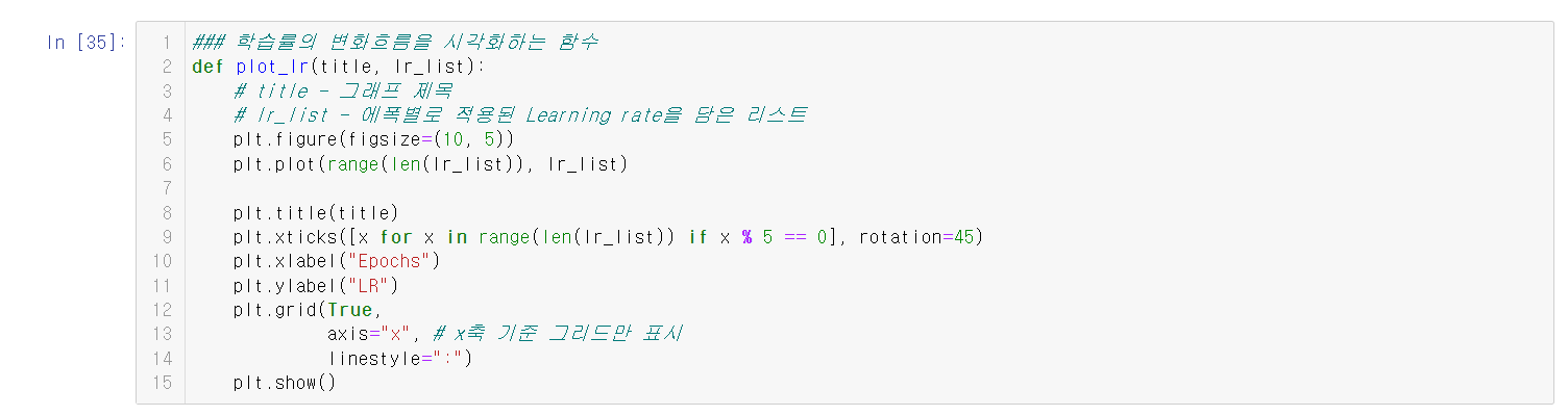

이 그래프의 내용은 다음과 같다.
13.stepLR
Learning rate decay와는 사뭇 다른 내용이다.
자세한 것은 아래 사진을 보자.
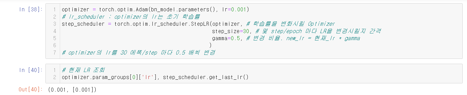
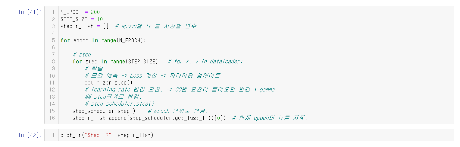
그래프는 아래와 같이 나온다.
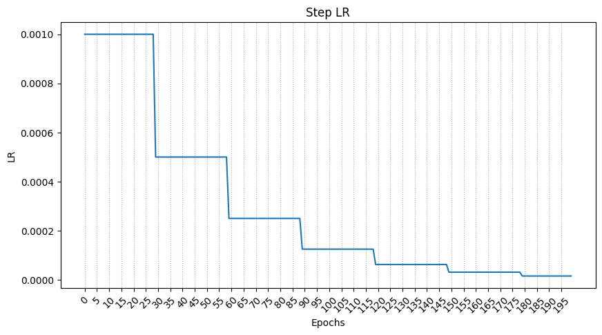
stepLR이 Learning rate decay와 다른 이유는
epochs가 늘어날 수록 lr은 줄어들기 때문이다.
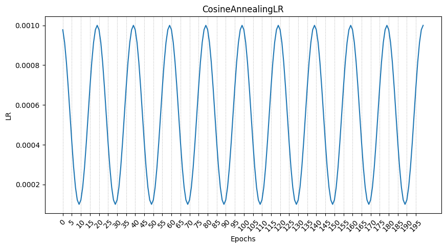
14.CosineAnnealingLR
간단하다. 코사인을 그리면서 학습률을 변동시킨다.
단순히 감소시키기 보다는 늘렸다가 줄였다가를 하면서 최적점을 찾아가는
알고리즘을 많이 사용하는게 요즘 트렌드인데,
이에 찰떡인게 바로 CosineAnnealingLR이다.

그래프의 결과는 다음과 같다.
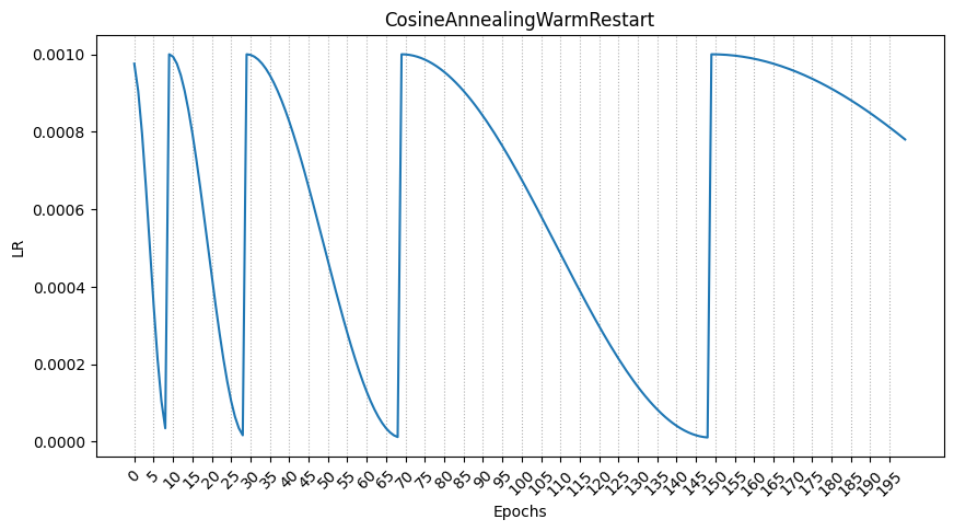
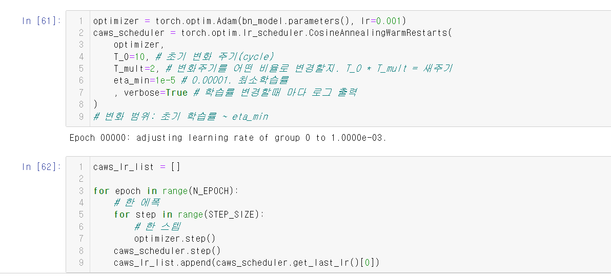
15.CosineAnnealingWarmRestarts
cosine annealing의 스케쥴링에 cosine 주기의 에폭을 점점 늘리거나 줄일 수 있다.
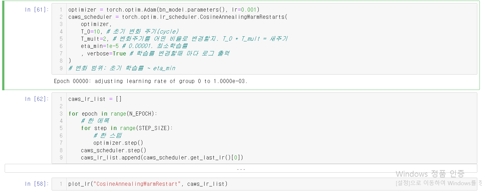
그래프의 결과는 다음과 같다.