
머신러닝·딥러닝 문제해결 전략 책을 읽으면서
Kaggle 경진대회 코드와 문제해결 전략을 정리한 글
8장 포르투 세구로 안전 운전자 예측 경진대회 - 탐색적 데이터 분석
경진대회 이해
- 포르투 세구로 보험사에서 제공한 고객 데이터를 활용해 운전자가 보험을 청구할 확률 예측
- 주어진 데이터는 포르투 세구로 브라질 보험 회사가 보유한 고객 데이터로 고객을 특정할 수 없도록 비식별화되어 있음
- 한편, 주어진 데이터는 결측값이 많으며 -1로 기록되어 있음
- 타깃값은 0 또는 1, 두 개이므로 본 경진대회는 이진분류 문제에 속함
- 값이 0이면 운전자가 보험금을 청구하지 않는다는 뜻이고 1이면 청구한다는 뜻
데이터 둘러보기
import pandas as pd

# 데이터 경로
data_path = '/kaggle/input/porto-seguro-safe-driver-prediction/'

train = pd.read_csv(data_path + 'train.csv', index_col='id')
test = pd.read_csv(data_path + 'test.csv', index_col='id')
submission = pd.read_csv(data_path + 'sample_submission.csv', index_col='id')train.shape, test.shape((595212, 58), (892816, 57))훈련 데이터는 약 59만개, 테스트 데이터는 약 89만개로 훈련 데이터보다 테스트 데이터가 더 많음.
타깃값을 제외하면 피처는 총 57개.
지금까지의 경진대회에 비해 데이터가 크고 피처 수도 많음
train.head()| target | ps_ind_01 | ps_ind_02_cat | ps_ind_03 | ps_ind_04_cat | ps_ind_05_cat | ps_ind_06_bin | ps_ind_07_bin | ps_ind_08_bin | ps_ind_09_bin | ... | ps_calc_11 | ps_calc_12 | ps_calc_13 | ps_calc_14 | ps_calc_15_bin | ps_calc_16_bin | ps_calc_17_bin | ps_calc_18_bin | ps_calc_19_bin | ps_calc_20_bin | |
|---|---|---|---|---|---|---|---|---|---|---|---|---|---|---|---|---|---|---|---|---|---|
| id | |||||||||||||||||||||
| 7 | 0 | 2 | 2 | 5 | 1 | 0 | 0 | 1 | 0 | 0 | ... | 9 | 1 | 5 | 8 | 0 | 1 | 1 | 0 | 0 | 1 |
| 9 | 0 | 1 | 1 | 7 | 0 | 0 | 0 | 0 | 1 | 0 | ... | 3 | 1 | 1 | 9 | 0 | 1 | 1 | 0 | 1 | 0 |
| 13 | 0 | 5 | 4 | 9 | 1 | 0 | 0 | 0 | 1 | 0 | ... | 4 | 2 | 7 | 7 | 0 | 1 | 1 | 0 | 1 | 0 |
| 16 | 0 | 0 | 1 | 2 | 0 | 0 | 1 | 0 | 0 | 0 | ... | 2 | 2 | 4 | 9 | 0 | 0 | 0 | 0 | 0 | 0 |
| 17 | 0 | 0 | 2 | 0 | 1 | 0 | 1 | 0 | 0 | 0 | ... | 3 | 1 | 1 | 3 | 0 | 0 | 0 | 1 | 1 | 0 |
5 rows × 58 columns
test.head()| ps_ind_01 | ps_ind_02_cat | ps_ind_03 | ps_ind_04_cat | ps_ind_05_cat | ps_ind_06_bin | ps_ind_07_bin | ps_ind_08_bin | ps_ind_09_bin | ps_ind_10_bin | ... | ps_calc_11 | ps_calc_12 | ps_calc_13 | ps_calc_14 | ps_calc_15_bin | ps_calc_16_bin | ps_calc_17_bin | ps_calc_18_bin | ps_calc_19_bin | ps_calc_20_bin | |
|---|---|---|---|---|---|---|---|---|---|---|---|---|---|---|---|---|---|---|---|---|---|
| id | |||||||||||||||||||||
| 0 | 0 | 1 | 8 | 1 | 0 | 0 | 1 | 0 | 0 | 0 | ... | 1 | 1 | 1 | 12 | 0 | 1 | 1 | 0 | 0 | 1 |
| 1 | 4 | 2 | 5 | 1 | 0 | 0 | 0 | 0 | 1 | 0 | ... | 2 | 0 | 3 | 10 | 0 | 0 | 1 | 1 | 0 | 1 |
| 2 | 5 | 1 | 3 | 0 | 0 | 0 | 0 | 0 | 1 | 0 | ... | 4 | 0 | 2 | 4 | 0 | 0 | 0 | 0 | 0 | 0 |
| 3 | 0 | 1 | 6 | 0 | 0 | 1 | 0 | 0 | 0 | 0 | ... | 5 | 1 | 0 | 5 | 1 | 0 | 1 | 0 | 0 | 0 |
| 4 | 5 | 1 | 7 | 0 | 0 | 0 | 0 | 0 | 1 | 0 | ... | 4 | 0 | 0 | 4 | 0 | 1 | 1 | 0 | 0 | 1 |
5 rows × 57 columns
submission.head()| target | |
|---|---|
| id | |
| 0 | 0.0364 |
| 1 | 0.0364 |
| 2 | 0.0364 |
| 3 | 0.0364 |
| 4 | 0.0364 |
타깃값 확률은 0.0364로 일괄 입력되어 있음.
7장과 마찬가지로 본 경진대회에서 예측해야 하는 값은 '타깃값이 1일 확률'임.
타깃값 0은 운전자가 보험금을 청구하지 않는 경우, 타깃값 1은 청구하는 경우를 의미.
train.info()<class 'pandas.core.frame.DataFrame'>
Int64Index: 595212 entries, 7 to 1488027
Data columns (total 58 columns):
# Column Non-Null Count Dtype
--- ------ -------------- -----
0 target 595212 non-null int64
1 ps_ind_01 595212 non-null int64
2 ps_ind_02_cat 595212 non-null int64
3 ps_ind_03 595212 non-null int64
4 ps_ind_04_cat 595212 non-null int64
5 ps_ind_05_cat 595212 non-null int64
6 ps_ind_06_bin 595212 non-null int64
7 ps_ind_07_bin 595212 non-null int64
8 ps_ind_08_bin 595212 non-null int64
9 ps_ind_09_bin 595212 non-null int64
10 ps_ind_10_bin 595212 non-null int64
11 ps_ind_11_bin 595212 non-null int64
12 ps_ind_12_bin 595212 non-null int64
13 ps_ind_13_bin 595212 non-null int64
14 ps_ind_14 595212 non-null int64
15 ps_ind_15 595212 non-null int64
16 ps_ind_16_bin 595212 non-null int64
17 ps_ind_17_bin 595212 non-null int64
18 ps_ind_18_bin 595212 non-null int64
19 ps_reg_01 595212 non-null float64
20 ps_reg_02 595212 non-null float64
21 ps_reg_03 595212 non-null float64
22 ps_car_01_cat 595212 non-null int64
23 ps_car_02_cat 595212 non-null int64
24 ps_car_03_cat 595212 non-null int64
25 ps_car_04_cat 595212 non-null int64
26 ps_car_05_cat 595212 non-null int64
27 ps_car_06_cat 595212 non-null int64
28 ps_car_07_cat 595212 non-null int64
29 ps_car_08_cat 595212 non-null int64
30 ps_car_09_cat 595212 non-null int64
31 ps_car_10_cat 595212 non-null int64
32 ps_car_11_cat 595212 non-null int64
33 ps_car_11 595212 non-null int64
34 ps_car_12 595212 non-null float64
35 ps_car_13 595212 non-null float64
36 ps_car_14 595212 non-null float64
37 ps_car_15 595212 non-null float64
38 ps_calc_01 595212 non-null float64
39 ps_calc_02 595212 non-null float64
40 ps_calc_03 595212 non-null float64
41 ps_calc_04 595212 non-null int64
42 ps_calc_05 595212 non-null int64
43 ps_calc_06 595212 non-null int64
44 ps_calc_07 595212 non-null int64
45 ps_calc_08 595212 non-null int64
46 ps_calc_09 595212 non-null int64
47 ps_calc_10 595212 non-null int64
48 ps_calc_11 595212 non-null int64
49 ps_calc_12 595212 non-null int64
50 ps_calc_13 595212 non-null int64
51 ps_calc_14 595212 non-null int64
52 ps_calc_15_bin 595212 non-null int64
53 ps_calc_16_bin 595212 non-null int64
54 ps_calc_17_bin 595212 non-null int64
55 ps_calc_18_bin 595212 non-null int64
56 ps_calc_19_bin 595212 non-null int64
57 ps_calc_20_bin 595212 non-null int64
dtypes: float64(10), int64(48)
memory usage: 267.9 MB- 데이터 타입은 int64와 float64 중 하나
- 피처명은 비식별화되어 있어서 어떤 의미인지 알 수 없지만 일정한 형식이 있음
- 피처명 형식 :
ps_[분류]_[분류별 일련번호]_[데이터 종류]- 분류로는 ind, reg, car, calc가 있으며 분류 다음엔 해당 분류에서의 일련번호가 나옴
- 마지막은 데이터 종류로 bin이면 이진 피처, cat이면 명목형 피처, 생략되어 있으면 순서형 또는 연속형 피처임
- 분류와 일련번호는 비식별화되어 있어서 어떠한 정보도 얻지 못하며 데이터 종류에서만 유의미한 정보를 얻을 수 있음
- 결측값은 -1로 입력되어 있기 때문에 피처별 결측값 수를 파악하기 위해 -1를 np.NaN으로 변환한 다음 개수를 셈
- 또한 피처가 많으므로 missingno 패키지를 사용하여 결측값을 시각화
import numpy as np
import missingno as msno

# 훈련 데이터 복사본에서 -1을 np.NaN로 변환
train_copy = train.copy().replace(-1, np.NaN)

# 결측값 시각화(처음 28개만)
msno.bar(df=train_copy.iloc[:, 1:29], figsize=(13, 6))<AxesSubplot:>
막대 그래프 높이가 낮을수록 결측값이 많다는 뜻
그래프 아래 피처명이 기재되어 있고 그래프 위에는 정상 값이 몇 개인지 표시되어 있음.
ps_reg_03, ps_car_03_cat, ps_car_05_cat 피처에 결측값이 많음
# 나머지 피처들의 결측값
msno.bar(df=train_copy.iloc[:, 29:], figsize=(13, 6))<AxesSubplot:>
ps_car_14에 결측값이 조금 있고 나머지 피처에는 없음
결측값 매트릭스 형태로 시각화하기
bar() 대신 matrix() 함수를 사용하면 결측값을 매트릭스 형태로 시각화할 수도 있음
msno.matrix(df=train_copy.iloc[:, 1:29], figsize=(13, 6))<AxesSubplot:>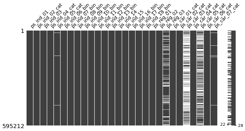
오른쪽 막대는 결측값의 상대적인 분포를 보여줌
검은색으로 뾰족하게 튀어나온 부분이 결측값이 몰려있는 행을 의미함
왼쪽에 표시된 22는 결측값이 없는 열 개수를, 오른쪽의 28은 전체 열 개수를 뜻함
피처 요약표
- 피처 종류가 다양하니 한눈에 파악할 수 있게 피처 요약표를 만드는 것이 좋음
- 피처 요약표가 있으면 데이터 관리도 편하고, 추후 그래프를 그릴 때도 활용할 수 있음
- 7장에서 만든 피처 요약표는 데이터 타입, 결측값 개수, 고윳값 개수, 1~3행에 입력된 값을 보여줬지만
- 본 경진대회에서 제공한 데이터는 숫자로 구성돼 있어 1~3행에 입력된 값은 추가하지 않고
- 시각화 시 피처를 추출하는 데 필요한 데이터 종류를 추가하도록 함
def resumetable(df):
    print(f'데이터셋 형상: {df.shape}')
    summary = pd.DataFrame(df.dtypes, columns=['데이터 타입'])
    summary['결측값 개수'] = (df == -1).sum().values  # 피처별 -1 개수
    summary['고윳값 개수'] = df.nunique().values
    summary['데이터 종류'] = None
    for col in df.columns:
        if 'bin' in col or col == 'target':
            summary.loc[col, '데이터 종류'] = '이진형'
        elif 'cat' in col:
            summary.loc[col, '데이터 종류'] = '명목형'
        elif df[col].dtype == float:
            summary.loc[col, '데이터 종류'] = '연속형'
        elif df[col].dtype == int:
            summary.loc[col, '데이터 종류'] = '순서형'

return summary- (df == -1).sum().values 코드로 피처별 -1 개수(결측값 개수)를 구함
- for문을 순회하며 데이터 종류 추가.
- 피처명에 'bin'이 포함돼 있거나 타깃 열이면 이진형 데이터
- 피처명에 'cat'이 포함돼 있으면 명목형 데이터
- 데이터 타입이 float면 연속형 데이터
- 데이터 타입이 int면 순서형 데이터
summary = resumetable(train)
summary
데이터셋 형상: (595212, 58)| 데이터 타입 | 결측값 개수 | 고윳값 개수 | 데이터 종류 | |
|---|---|---|---|---|
| target | int64 | 0 | 2 | 이진형 |
| ps_ind_01 | int64 | 0 | 8 | 순서형 |
| ps_ind_02_cat | int64 | 216 | 5 | 명목형 |
| ps_ind_03 | int64 | 0 | 12 | 순서형 |
| ps_ind_04_cat | int64 | 83 | 3 | 명목형 |
| ps_ind_05_cat | int64 | 5809 | 8 | 명목형 |
| ps_ind_06_bin | int64 | 0 | 2 | 이진형 |
| ps_ind_07_bin | int64 | 0 | 2 | 이진형 |
| ps_ind_08_bin | int64 | 0 | 2 | 이진형 |
| ps_ind_09_bin | int64 | 0 | 2 | 이진형 |
| ps_ind_10_bin | int64 | 0 | 2 | 이진형 |
| ps_ind_11_bin | int64 | 0 | 2 | 이진형 |
| ps_ind_12_bin | int64 | 0 | 2 | 이진형 |
| ps_ind_13_bin | int64 | 0 | 2 | 이진형 |
| ps_ind_14 | int64 | 0 | 5 | 순서형 |
| ps_ind_15 | int64 | 0 | 14 | 순서형 |
| ps_ind_16_bin | int64 | 0 | 2 | 이진형 |
| ps_ind_17_bin | int64 | 0 | 2 | 이진형 |
| ps_ind_18_bin | int64 | 0 | 2 | 이진형 |
| ps_reg_01 | float64 | 0 | 10 | 연속형 |
| ps_reg_02 | float64 | 0 | 19 | 연속형 |
| ps_reg_03 | float64 | 107772 | 5013 | 연속형 |
| ps_car_01_cat | int64 | 107 | 13 | 명목형 |
| ps_car_02_cat | int64 | 5 | 3 | 명목형 |
| ps_car_03_cat | int64 | 411231 | 3 | 명목형 |
| ps_car_04_cat | int64 | 0 | 10 | 명목형 |
| ps_car_05_cat | int64 | 266551 | 3 | 명목형 |
| ps_car_06_cat | int64 | 0 | 18 | 명목형 |
| ps_car_07_cat | int64 | 11489 | 3 | 명목형 |
| ps_car_08_cat | int64 | 0 | 2 | 명목형 |
| ps_car_09_cat | int64 | 569 | 6 | 명목형 |
| ps_car_10_cat | int64 | 0 | 3 | 명목형 |
| ps_car_11_cat | int64 | 0 | 104 | 명목형 |
| ps_car_11 | int64 | 5 | 5 | 순서형 |
| ps_car_12 | float64 | 1 | 184 | 연속형 |
| ps_car_13 | float64 | 0 | 70482 | 연속형 |
| ps_car_14 | float64 | 42620 | 850 | 연속형 |
| ps_car_15 | float64 | 0 | 15 | 연속형 |
| ps_calc_01 | float64 | 0 | 10 | 연속형 |
| ps_calc_02 | float64 | 0 | 10 | 연속형 |
| ps_calc_03 | float64 | 0 | 10 | 연속형 |
| ps_calc_04 | int64 | 0 | 6 | 순서형 |
| ps_calc_05 | int64 | 0 | 7 | 순서형 |
| ps_calc_06 | int64 | 0 | 11 | 순서형 |
| ps_calc_07 | int64 | 0 | 10 | 순서형 |
| ps_calc_08 | int64 | 0 | 11 | 순서형 |
| ps_calc_09 | int64 | 0 | 8 | 순서형 |
| ps_calc_10 | int64 | 0 | 26 | 순서형 |
| ps_calc_11 | int64 | 0 | 20 | 순서형 |
| ps_calc_12 | int64 | 0 | 11 | 순서형 |
| ps_calc_13 | int64 | 0 | 14 | 순서형 |
| ps_calc_14 | int64 | 0 | 24 | 순서형 |
| ps_calc_15_bin | int64 | 0 | 2 | 이진형 |
| ps_calc_16_bin | int64 | 0 | 2 | 이진형 |
| ps_calc_17_bin | int64 | 0 | 2 | 이진형 |
| ps_calc_18_bin | int64 | 0 | 2 | 이진형 |
| ps_calc_19_bin | int64 | 0 | 2 | 이진형 |
| ps_calc_20_bin | int64 | 0 | 2 | 이진형 |
# 피처 요약표에서 명목형 피처 추출
summary[summary['데이터 종류'] == '명목형'].index
Index(['ps_ind_02_cat', 'ps_ind_04_cat', 'ps_ind_05_cat', 'ps_car_01_cat',
'ps_car_02_cat', 'ps_car_03_cat', 'ps_car_04_cat', 'ps_car_05_cat',
'ps_car_06_cat', 'ps_car_07_cat', 'ps_car_08_cat', 'ps_car_09_cat',
'ps_car_10_cat', 'ps_car_11_cat'],
dtype='object')# 피처 요약표에서 데이터 타입이 실수형인 피처 추출
summary[summary['데이터 타입'] == 'float64'].indexIndex(['ps_reg_01', 'ps_reg_02', 'ps_reg_03', 'ps_car_12', 'ps_car_13',
'ps_car_14', 'ps_car_15', 'ps_calc_01', 'ps_calc_02', 'ps_calc_03'],
dtype='object')데이터 시각화
- 데이터 시각화를 통해 모델링에 필요한 피처는 무엇이고, 필요 없는 피처는 무엇인지 선별
- 먼저 타깃값 분포를 활용해 타깃값이 얼마나 불균형한지 알아보고
- 이진 피처, 명목형 피처, 순서형 피처의 고윳값별 타깃값 비율 알아보기
import seaborn as sns
import matplotlib as mpl
import matplotlib.pyplot as plt
%matplotlib inline
타깃값 분포
def write_percent(ax, total_size):
    '''도형 객체를 순회하며 막대 그래프 상단에 타깃값 비율 표시'''
    for patch in ax.patches:
        height = patch.get_height()       # 도형 높이 (데이터 개수)
        width = patch.get_width()        # 도형 너비
        left_coord = patch.get_x()       # 도형 왼쪽 테두리의 x축 위치
        percent = height/total_size*100  # 타깃값 비율

        # (x, y) 좌표에 텍스트 입력
        ax.text(left_coord + width/2.0,     # x축 위치
                height + total_size*0.001,  # y축 위치
                '{:1.1f}%'.format(percent),  # 입력 텍스트
                ha='center')                # 가운데 정렬

mpl.rc('font', size=15)
plt.figure(figsize=(7, 6))

ax = sns.countplot(x='target', data=train)
write_percent(ax, len(train))  # 비율 표시
ax.set_title('Target Distribution')
Text(0.5, 1.0, 'Target Distribution')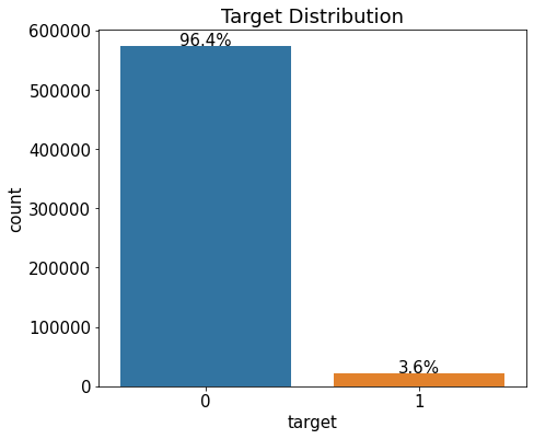
타깃값 0은 96.4%를 차지하며 1은 단 3.6%만을 차지함.
전체 운전자 중 3.6%만 보험금을 청구했다는 뜻.
→ 타깃값 불균형
-
타깃값이 불균형하기 때문에 비율이 작은 타깃값 1을 잘 예측하는 게 중요함
-
따라서 이번에는 각 피처의 분포를 알아보기 보다는, 각 피처의 고윳값별 타깃값 1 비율을 알아보도록 함
-
고윳값별 타깃값 1 비율을 통해 해당 피처가 모델링에 필요한 피처인지 확인할 수 있음
-
예컨대 피처 A에 고윳값 a, b가 있다고 하면 이때 고윳값 a, b별로 타깃값 1 비율이 얼마나 되는지 살펴보려는 것
-
고윳값별로 타깃값 1 비율이 똑같거나 통계적 유효성이 떨어지면, 즉 통계적으로 유의미한 차이가 없다면 피처 A로는 무언가를 분별하기 어려우므로 예측에 도움되지 않음
-
다시 말해, 고윳값에 따라 타깃값 비율이 달라야 그 피처가 타깃값 예측에 도움을 줌
-
타깃값 1 비율의 통계적 유효성이 떨어져도 불필요한 피처가 될 수 있음
-
통계적 유효성은 barplot()을 그릴 때 나타나는 신뢰구간으로 판단함
-
신뢰구간이 좁다면 통계적으로 어느 정도 유효하다고 보고, 구간이 넓다면 신뢰하기 어렵다고 보는 것
-
통계적 유효성이 높아야(신뢰구간이 좁아야) 모델링에 도움이 됨
종합하면, 고윳값별 타깃값 1 비율이 충분히 차이가 나고 신뢰구간도 작은 피처여야 모델링에 도움이 됨
그렇지 않은 피처는 제거하는 게 좋음
이진 피처
- 이상의 내용에 유념해 이진 피처의 고윳값별 타깃값 비율 구하기
import matplotlib.gridspec as gridspec

def plot_target_ratio_by_features(df, features, num_rows, num_cols, size=(12, 18)):
    mpl.rc('font', size=9)
    plt.figure(figsize=size)                       # 전체 Figure 크기 설정
    grid = gridspec.GridSpec(num_rows, num_cols)   # 서브플롯 배치
    plt.subplots_adjust(wspace=0.3, hspace=0.3)    # 서브플롯 좌우/상하 여백 설정

    for idx, feature in enumerate(features):
        ax = plt.subplot(grid[idx])
        # ax축에 고윳값별 타깃값 1 비율을 막대 그래프로 그리기
        sns.barplot(x=feature, y='target', data=df, palette='Set2', ax=ax)
bin_features = summary[summary['데이터 종류'] == '이진형'].index # 이진 피처
# 이진 피처 고윳값별 타깃값 1 비율을 막대 그래프로 그리기
plot_target_ratio_by_features(train, bin_features, 6, 3) # 6행 3열 배치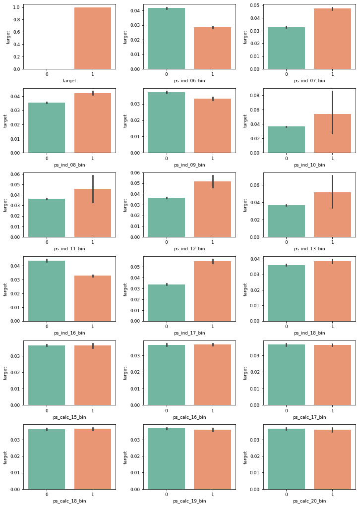
ps_ind_06_bin 피처의 고윳값별 타깃값 비율
| 고윳값 | 타깃값 1 비율 | 타깃값 0 비율 |
|---|---|---|
| 0 | 4% | 96% |
| 1 | 2.8% | 97.2% |
ps_ind_06_bin 피처는 고윳값별로 타깃값 비율이 다르므로 타깃값을 추정하는 예측력이 있음. 게다가 신뢰구간도 좁기 때문에 모델링에 도움이 되는 피처.
제거해야 할 이진 피처
| 서브플롯 위치 | 피처명 | 제거해야 하는 이유 |
|---|---|---|
| 1행 2열~2행 2열 | ps_ind_10_bin ~ ps_ind_13_bin | 신뢰구간이 넓어 통계적 유효성이 떨어짐 |
| 4행 0열~5행 2열 | ps_calc_15_bin ~ ps_calc_20_bin | 고윳값별 타깃값 비율 차이가 없어 타깃값 예측력이 없음 |
여기서 주목할 점은 calc 분류의 이진 피처는 모두 타깃값 비율에 차이가 없다는 사실
신뢰구간이 얼마나 넓어야 제거할 피처로 볼지, 고윳값별 타깃값 비율이 얼마나 달라야 제거할 피처로 볼지는 사람마다 다르게 판단할 수 있음.
또한 제거할 피처를 찾기 위한 다른 방법도 많으므로 이런 논리로 제거할 피처를 골라낼 수 있다는 정도로 알아두기
명목형 피처
- 명목형 피처의 고윳값별 타깃값 비율 구하기
nom_features = summary[summary['데이터 종류'] == '명목형'].index  # 명목형 피처

plot_target_ratio_by_features(train, nom_features, 7, 2)  # 7행 2열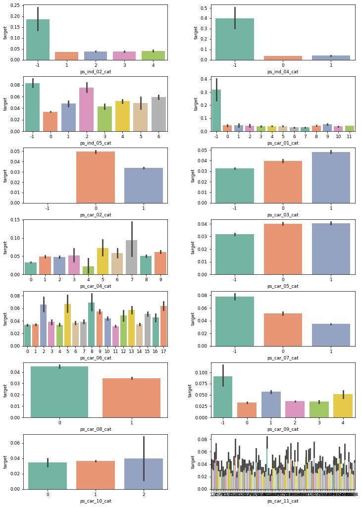
ps_ind_02_cat피처의 경우 결측값 -1이 다른 고윳값들보다 타깃값 1 비율이 큼.- 신뢰구간이 넓다는 점을 감안해도 비율이 확실히 큼
- 이런 상황에서 결측값을 다른 값으로 대체하면 모델 성능이 나빠질 수 있음
- 결측값 자체가 타깃값에 대한 예측력이 있기 때문
- 따라서 결측값을 그대로 두고 모델링
- -1도 하나의 고윳값이라고 간주하는 것
ps_car_02_cat피처의 경우 -1일 때 타깃값 1 비율은 0%- 이 경우만 놓고 볼 때
ps_car_02_cat피처 값이 -1이면 타깃값이 0이라고 판단할 수 있음 - 이 역시 결측값이 타깃값을 예측하는 데 도움을 줌
- 결측값을 포함하는 다른 피처도 비슷한 양상을 보임
- 이 경우만 놓고 볼 때
→ 결측값 자체에 타깃값 예측력이 있다면 고윳값으로 간주 (결측값 처리 필요 없음)
명목형 피처 중 제거할 피처는 없음
ps_ind_02_cat,ps_ind_04_cat,ps_cat_01_cat그래프를 보면- -1을 제외하고 나머지 고윳값은 타깃값 1 비율이 비슷하며 -1일 때의 신뢰구간이 상대적으로 넓음
- 그렇더라도 -1의 신뢰하한과 다른 고윳값들의 신뢰상한 간 차이가 큼
- 따라서 -1의 신뢰구간이 넓다는 점을 감안해도 -1과 다른 고윳값들 간 타깃값 1 비율에 차이가 있음
- 즉, 고윳값 간 타깃값 1 비율에 차이가 있으므로 모델링에 필요한 피처
ps_car_10_cat피처의 경우- 세 고윳값은 타깃값 1의 평균 비율이 비슷하고 고윳값 2의 신뢰구간이 유독 넓음
- 이 피처를 제거해야 하는가는 애매함
- 실제 상위권 캐글러 중 이 피처를 제거한 사람도 있고 그대로 둔 사람도 있음
- 이럴 때는 해당 피처를 제거한 경우와 제거하지 않은 경우에 성능이 어떻게 다른지 비교해보는 것도 좋은 방법
- 책에서는 제거하지 않은 경우에 성능이 더 좋았다고 하므로 제거하지 않도록 함
순서형 피처
- 순서형 피처의 고윳값별 타깃값 비율 구하기
ord_features = summary[summary['데이터 종류'] == '순서형'].index  # 순서형 피처

plot_target_ratio_by_features(train, ord_features, 8, 2, (12, 20))  # 8행 2열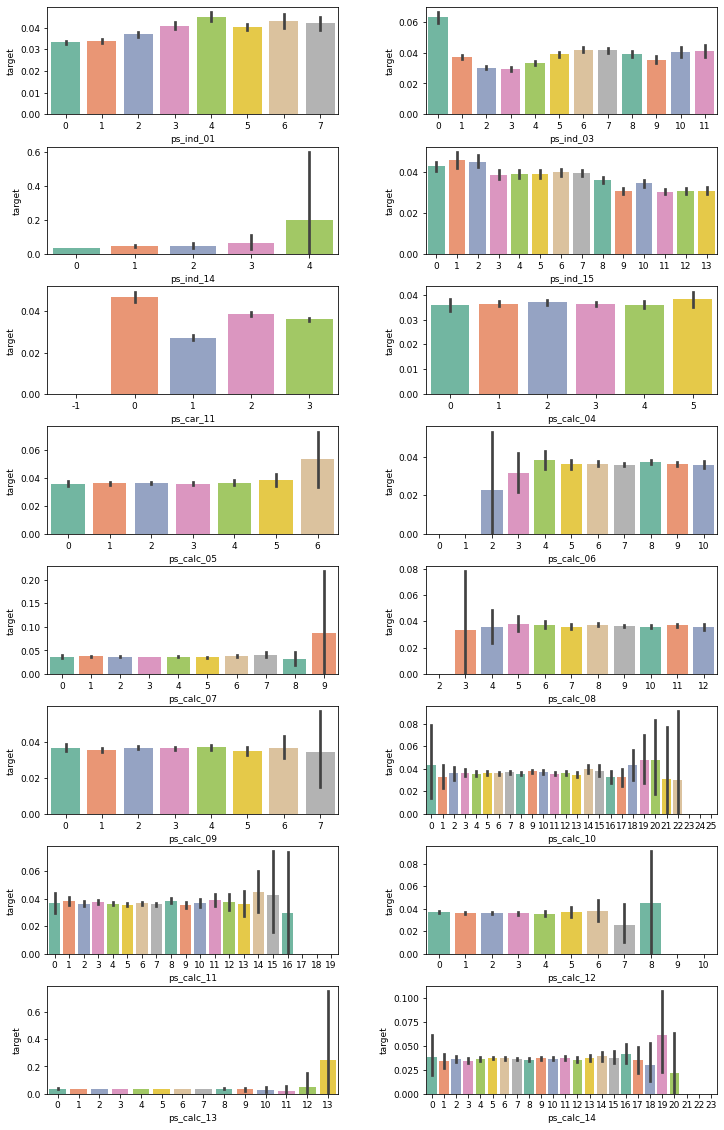
ps_ind_14피처 그래프를 보면 고윳값 0, 1, 2, 3의 타깃값 비율은 큰 차이가 없고, 고윳값 4의 신뢰구간은 넓음- 신뢰구간이 상당히 넓어 통계적 유효성이 떨어지므로
ps_ind_14피처는 제거
- 신뢰구간이 상당히 넓어 통계적 유효성이 떨어지므로
ps_calc_04부터ps_calc_14까지는 모두 고윳값별 타깃값 비율이 거의 비슷함- 타깃값 비율이 다른 고윳값도 있긴 하지만 그 고윳값은 신뢰구간이 넓어 통계적 유효성이 떨어짐
- 따라서 이 피처들은 모두 제거하도록 함
- 앞서 '이진 피처' 절에서 calc 분류에 속하는 이진 피처는 모두 제거하기로 했는데 순서형 피처에서도 마찬가지로 calc 분류의 모든 피처를 제거하게 됨
제거해야 할 순서형 피처
| 서브플롯 위치 | 피처명 | 제거해야 하는 이유 |
|---|---|---|
| 1행 0열 | ps_ind_14 | 타깃값 비율의 신뢰구간이 넓어 통계적 유효성이 떨어짐 |
| 2행 1열~7행 1열 | ps_calc_04 ~ ps_calc_14 | 고윳값별 타깃값 비율 차이가 없음 타깃값 비율이 다르더라도 신뢰구간이 넓어 통계적 유효성이 떨어짐 |
연속형 피처
- 연속형 피처는 연속된 값이므로 고윳값이 굉장히 많아서 고윳값별 타깃값 1 비율을 구하기 힘듬
- 그렇기 때문에 값을 몇 개의 구간으로 나눠 구간별 타깃값 1 비율을 알아봄
# 판다스의 cut() 함수를 활용하여 여러 개의 값을 3개 구간으로 나누는 예
# 함수의 첫 번째 인수가 값들의 리스트이며, 두 번째 인수가 나눌 구간의 개수
pd.cut([1.0, 1.5, 2.1, 2.7, 3.5, 4.0], 3)
[(0.997, 2.0], (0.997, 2.0], (2.0, 3.0], (2.0, 3.0], (3.0, 4.0], (3.0, 4.0]]
Categories (3, interval[float64, right]): [(0.997, 2.0] < (2.0, 3.0] < (3.0, 4.0]]cont_features = summary[summary['데이터 종류'] == '연속형'].index # 연속형 피처
plt.figure(figsize=(12, 26)) # Figure 크기 설정
grid = gridspec.GridSpec(5, 2) # GridSpec 객체 생성
plt.subplots_adjust(wspace=0.2 , hspace=0.4) # 서브플롯 간 여백 설정
for idx, cont_feature in enumerate(cont_features):
# 값을 5개 구간으로 나누기
train[cont_feature] = pd.cut(train[cont_feature], 5)
ax = plt.subplot(grid[idx]) # 분포도를 그릴 서브플롯 설정
sns.barplot(x=cont_feature, y='target', data=train, palette='Set2', ax=ax)
ax.tick_params(axis='x', labelrotation=10) # x축 라벨 회전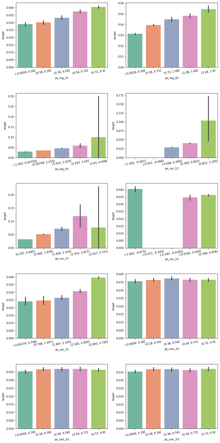
제거해야 할 연속형 피처
| 서브플롯 위치 | 피처명 | 제거해야 하는 이유 |
|---|---|---|
| 3행 1열~4행 1열 | ps_calc_01~ps_calc_03 | 구간별 타깃값 비율 차이가 없음 |
- 이로써 calc 분류의 피처는 데이터 종류에 상관없이 모두 제거해야 한다는 사실을 알게 됨
- 이 피처들은 고윳값 혹은 구간별로 타깃값 비율이 거의 같음 → 타깃값을 구분하는 예측 능력이 떨어진다는 뜻
연속형 피처Ⅱ
- 연속형 피처 간 '상관관계' 파악
- 상관관계가 강한 피처들은 타깃값 예측력도 비슷하므로 둘 중 하나만 남겨두는 것이 좋음
상관관계가 얼마나 강한 피처를 제거해야 하는가?
상관계수가 얼마 이상일 때 제거하는 게 좋은지 정해진 기준은 없으며 상황과 모델에 따라 다름
더불어, 강한 상관관계를 보이는 두 피처 중 하나를 제거한다고 해서 반드시 성능이 향상되는 것도 아님
'고려해볼 만한 요소'정도로 생각하면 되고 상관계수가 0.8 이상이라면 제거를 고려해보는 것도 좋은 방법
피처 간 상관관계를 파악하기 위해 히트맵 그려보기
- 결측값이 있으면 상관관계를 올바르게 구하지 못하므로 결측값을 제거하고 그려야 함
- 현재 피처에는 결측값이 있으므로 -1을 np.NaN으로 변환한 train_copy에서 np.NaN을 제거하도록 함
train_copy = train_copy.dropna() # np.NaN 값 삭제plt.figure(figsize=(10, 8))
cont_corr = train_copy[cont_features].corr() # 연속형 피처 간 상관관계
sns.heatmap(cont_corr, annot=True, cmap='OrRd') # 히트맵 그리기<AxesSubplot:>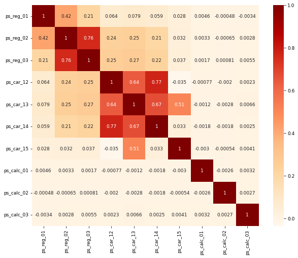
- 가장 강한 상관관계를 보이는
ps_car_12와ps_car_14피처 간 상관계수는 0.77 - 둘 중 하나를 제거해야 할 만큼 강한 상관관계를 보이는 것은 아니지만 테스트 결과
ps_cat_14피처를 제거하니 성능이 더 좋아짐 - 성능 향상을 위해
ps_cat_14피처를 추가로 제거하도록 함 - 두 번째로 상관관계가 강한
ps_reg_02와ps_reg_03피처 간 상관계수는 0.76 - 이 경우는 테스트 결과 둘 중 하나를 제거하니 오히려 성능이 떨어지므로 그대로 남겨두도록 함
분석 정리 및 모델링 전략
분석 정리
- 6장과 7장의 경진대회에 비해 데이터가 크고 피처 수도 많음
- 피처명만으로 분류별 혹은 데이터 종류별 피처들을 구분해 추출해낼 수 있음
- 결측값 처리 : 결측값 자체에 타깃값 예측력이 있다면 고윳값으로 간주
- 결측값 처리 : 피처 간 상관관계 분석은 결측값 제거 후 수행
- 피처 제거 : 신뢰구간이 넓으면 통계적 유효성이 떨어져 믿을 수 없음 (
ps_ind_14,ps_calc_04~ps_calc_14) - 피처 제거 : 고윳값별 타깃값 비율에 차이가 없다면 타깃값 예측력이 없음 (
ps_calc_04~ps_calc_14) - 피처 제거 : (연속형 데이터의 경우) 구간별 타깃값 차이가 거의 없다면 타깃값 예측력이 없음 (
ps_calc_01~ps_calc_03) - 피처 제거 : 일반적으로 강한 상관관계를 보이는 두 피처가 있으면 둘 중 하나만 제거하는 게 좋음 (
ps_car_14)
모델링 전략
이번 장의 목표는 캐글에서 실제로 많이 활용되는 여러 가지 고급 모델링 기법 배우기
주요 키워드는 OOF 예측, 베이지안 최적화, LightGBM, XGBoost, 앙상블
- 베이스라인 모델 : LightGBM
- 훈련 및 예측 : OOF 예측 (과대적합 방지 + 앙상블 효과)
- 성능 개선Ⅰ : LightGBM 유지
- 피처 엔지니어링 : 파생 피처 추가
- 하이퍼파라미터 최적화 : 베이지안 최적화
- 성능 개선Ⅱ : XGBoost (모델만 변경)
- 성능 개선Ⅲ : LightGBM + XGBoost 앙상블
