05. 상관관계

5.1 피어슨 상관계수

가장 대표적으로 많이 사용하는 상관계수!

(왼쪽 그래프)

피어슨 상관계수란 ?

• 두 연속형 변수 간의 선형 관계를 측정하는 지표
• -1에서 1 사이의 값을 가지며
• 1은 완전한 양의 선형 관계
• -1은 완전한 음의 선형 관계
• 0은 선형 관계가 없음을 의미

실제 사례

🫡 선형적인 관계가 예상 될 때 사용(비선형적일 때는 사용 불가🔥)

• 공부 시간과 시험 점수 간의 상관관계 분석

<예시 코드>

import numpy as np
import pandas as pd
import matplotlib.pyplot as plt
import seaborn as sns
from scipy.stats import pearsonr

# 예시 데이터 생성
np.random.seed(0)
study_hours = np.random.rand(100) * 10
exam_scores = 3 * study_hours + np.random.randn(100) * 5

# 데이터프레임 생성
df = pd.DataFrame({'Study Hours': study_hours, 'Exam Scores': exam_scores})

# 피어슨 상관계수 계산
pearson_corr, _ = pearsonr(df['Study Hours'], df['Exam Scores'])
print(f"피어슨 상관계수: {pearson_corr}")

# 상관관계 히트맵 시각화
sns.heatmap(df.corr(), annot=True, cmap='coolwarm', vmin=-1, vmax=1)
plt.title('pearson coefficient heatmap')
plt.show()

5.2 비모수 상관계수

데이터가 정규분포를 따르지 않을 때 사용하는 상관계수!

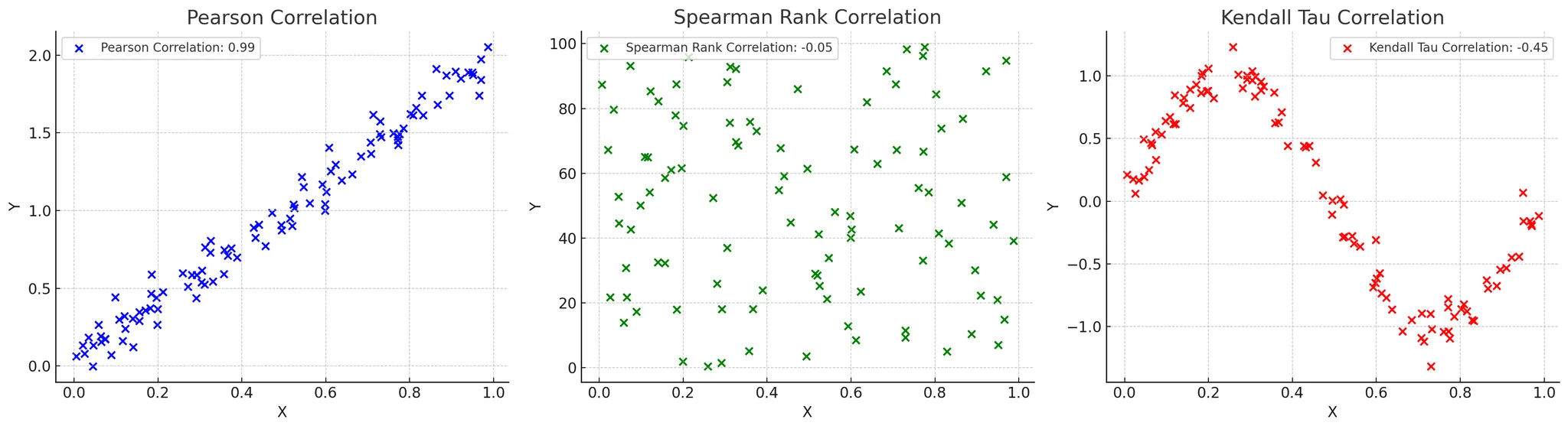
(가운데, 오른쪽 그래프)

비모수 상관계수란?

• 데이터가 정규분포를 따르지 않거나 변수들이 순서형 데이터일 때 사용하는 상관계수
• 데이터의 분포에 대한 가정 없이 두 변수 간의 상관관계를 측정할 때 사용
• 대표적으로 스피어만 상관계수와 켄달의 타우 상관계수가 있음

1. 스피어만 상관계수

• 두 변수의 순위 간의 일관성을 측정(두 변수의 순위 간의 상관 관계를 측정)
• 켄달의 타우 상관계수 보다 데이터 내 편차와 에러에 민감
• 값은 -1에서 1 사이로 해석

2. 켄달의 타우 상관계수

• 순위 간의 일치 쌍 및 불일치 쌍의 비율을 바탕으로 계산
• ex) 예를들어 사람의 키와 몸무게에 대해 상관계수를 알고자 할 때 키가 크고 몸무게도 더 나가면 일치 쌍에 해당, 키가 크지만 몸무게가 더 적으면 불일치 쌍에 해당 이들의 개수 비율로 상관계수를 결정
• 비선형 관계를 탐지하는 데 유용

실제 사례

🌝 1. 데이터의 분포에 대한 가정을 하지 못할 때
🌝 2. 순서형 데이터에서도 사용하고 싶을 때

<예시 코드>

from scipy.stats import spearmanr, kendalltau

# 예시 데이터 생성
np.random.seed(0)
customer_satisfaction = np.random.rand(100)
repurchase_intent = 3 * customer_satisfaction + np.random.randn(100) * 0.5

# 데이터프레임 생성
df = pd.DataFrame({'Customer Satisfaction': customer_satisfaction, 'Repurchase Intent': repurchase_intent})

# 스피어만 상관계수 계산
spearman_corr, _ = spearmanr(df['Customer Satisfaction'], df['Repurchase Intent'])
print(f"스피어만 상관계수: {spearman_corr}")

# 켄달의 타우 상관계수 계산
kendall_corr, _ = kendalltau(df['Customer Satisfaction'], df['Repurchase Intent'])
print(f"켄달의 타우 상관계수: {kendall_corr}")

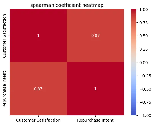
# 상관관계 히트맵 시각화
sns.heatmap(df.corr(method='spearman'), annot=True, cmap='coolwarm', vmin=-1, vmax=1)
plt.title('spearman coefficient heatmap')
plt.show()

5.3 상호정보 상관계수

상호정보를 이용한 변수끼리의 상관계수 계산!

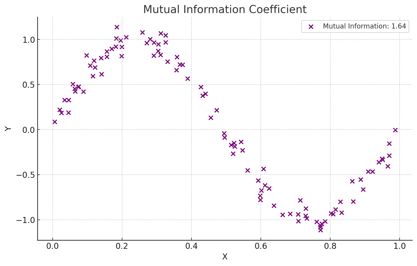
상호정보 상관계수란?

• 두 변수 간의 상호 정보를 측정
• 변수 간의 정보 의존성을 바탕으로 비선형 관계를 탐지
• 서로의 정보에 대한 불확실성을 줄이는 정도를 바탕으로 계산
• 범주형 데이터에 대해서도 적용 가능
• 상호정보 상관계수를 그림으로 확인해보기
  • 보라색 점들은 X와 Y 간의 비선형 관계를 나타냄
  • 상호 정보 값은 0.90으로 표시되어 있으며, 이는 두 변수 간의 강한 비선형 의존성을 의미

실제 사례

🌞 1.  두 변수가 범주형 변수일 때
🌞 2. 비선형적이고 복잡한 관계를 탐지하고자 할 때

import numpy as np
from sklearn.metrics import mutual_info_score

# 범주형 예제 데이터
X = np.array(['cat', 'dog', 'cat', 'cat', 'dog', 'dog', 'cat', 'dog', 'dog', 'cat'])
Y = np.array(['high', 'low', 'high', 'high', 'low', 'low', 'high', 'low', 'low', 'high'])

# 상호 정보량 계산
mi = mutual_info_score(X, Y)
print(f"Mutual Information (categorical): {mi}")

---

06. 가설검정의 주의점

6.1 재현가능성

우연히 결과가 나오는 것이 아닌, 항상 일관된 결과가 나오는지 확인해야 함!

재현가능성이란?

• 동일한 연구나 실험을 반복했을 때 일관된 결과가 나오는지 여부(연구의 신뢰성을 높이는 중요한 요소)
  ex) 신약을 개발할 때 실험실에서만 효과가 있는 것이 아니라 실제 상황에서도 일관된 결과가 나온다고 믿을 수 있기 때문에 개발 가능한 것
• 최근 p값에 대한 논쟁이 두드러지고 있음
  • p값을 사용하지 않는 것이 좋다
  • 유의수준을 0.05에서 변경하는 것이 좋다
• 가설검정 원리상의 문제나 가설검정의 잘못된 사용이 낮은 재현성으로 이어진다는 문제 발생
• 최근 논문을 다시 재현해서 실험을 해보는데 똑같은 결과가 안 나오는 사례가 많은… 재현성 위기가 문제가 되고 있음
• 결과가 재현되지 않는다면 해당 가설의 신뢰도가 떨어짐

재현성 위기의 원인은?

☑️ 실험 조건을 동일하게 조성하기 어려움

• 완전 동일하게 다시 똑같은 실험을 수행하는 것이 쉽지 않음
• 또한 가설검정 자체도 100% 검정력을 가진 것이 아니기 때문에 오차가 나타날 수 있음

☑️ 가설검정 사용방법에 있어서 잘못됨

• p값이 0.05가 유도되게끔 조작하는 것이 가능 (p해킹)
• 실제로는 통계적으로 아무 의미가 없음에도 의미가 있다고 해버리는 1종 오류를 저지를 수 있음
• 0.05라는 것은 100번 중에 5번 즉, 20번 중에 1번은 귀무가설이 옳음에도 불구하고 기각될 수 있음
• 유의수준으로 통제하는 것이 중요
• 하지만, 유의수준을 너무 낮추면 베타값이 커져버리는 문제 발생…
• 따라서, 어떤 논문에서는 유의수준을 0.005로 설정하면서 데이터 수를 70% 더 늘려서 베타 값도 컨트롤 하는 방향을 제안하기도 함
• 잘못된 가설을 세우더라도 우연히 0.05보다 낮아서 가설이 맞는것처럼 보일 수도 있음. 따라서 가능한 좋은 가설을 세우는 것도 중요

6.2 p-해킹

인위적으로 p-값을 낮추지 않을 수 있도록 조심해야 함!

p-해킹이란?

• 데이터 분석을 반복하여 p-값을 인위적으로 낮추는 행위
• 유의미한 결과를 얻기 위해 다양한 변수를 시도하거나, 데이터를 계속해서 분석하는 등의 방법을 포함
• p-해킹은 데이터 분석 결과의 신뢰성을 저하시킴

p-해킹은 언제 조심해야하는가?

🫵🏻 여러 가설 검정을 시도 할 때

• 여러 가설 검정을 시도하여 유의미한 p-값을 얻을 때까지 반복 분석하는 것을 조심
• p-해킹은 유의미한 결과를 얻기 위해 p-값이 0.05 이하인 결과만 선택적으로 보고하는 행위를 조심
• 데이터의 수를 늘리다보니 특정 데이터 수를 기록할때 잠깐 p값이 0.05 이하를 기록함으로 이를 바탕으로 대립가설 채택하는 것을 조심
• 즉, 결과를 보며 데이터 개수를 늘려서는 안됨
• 다양한 상황 중에서 p값이 유리하게 나오는 상황만 선별적으로 보고하는 것을 조심
• 다양한 변수를 건드리며 유리한 결과가 나올 때 다시 처음 부터 가설을 그 결과에 맞게 세우는 것
• 즉, 마음에 드는 상황만 골라서 보고해서도 안됨. 모든 결과를 다보고하거나 더 엄격한 추가실험을 수행
• 가능한 가설을 미리 세우고 검증하는 가설검증형 방식으로 분석을 해야 하며 만약 탐색적으로 분석한 경우 가능한 모든 변수를 보고하고 본페로니 보정과 같은 방법을 사용해야 함

6.3 선택적 보고

말 그대로 선택적으로 보고하는 것!

선택적 보고란?

• 유의미한 결과만을 보고하고, 유의미하지 않은 결과는 보고하지 않는 행위
• 이는 데이터 분석의 결과를 왜곡하고, 신뢰성을 저하시킴
  <예시>
  
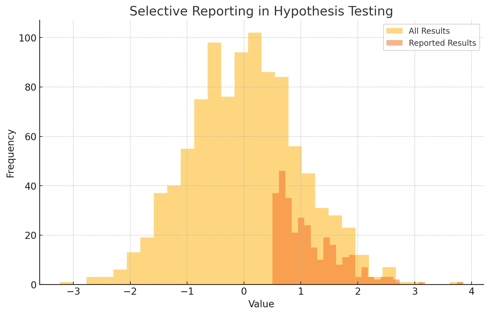
• 모든 결과와 선택적으로 보고된 결과를 히스토그램으로 나타냄
• 전체 결과와 보고된 결과의 분포가 다르면 선택적 보고의 가능성을 시사

선택적 보고는 언제 조심해야하는가?

☑️ 유의미한 결과만 공개 할 때

• 다수의 데이터 분석 중 유의미한 결과가 나온 실험만을 보고서에 작성하여 발표

☑️ 결과를 보면서 가설을 다시 새로 설정했는데 마치 처음부터 설정한 가설이라고 얘기할 때

• 미리 가설과 실험 방법등에 대해서 설정을 한 다음 연구를 수행하거나 연구하는 동안 얻어진 모든 변수와 결과에 대해서 공개하지 못할 때

6.4 자료수집 중단 시점 결정

원하는 결과가 나올 때 까지 자료를 수집하는 것을 조심!

자료수집 중단 시점 결정이란?

• 데이터 수집을 시작하기 전에 언제 수집을 중단할지 명확하게 결정하지 않으면, 원하는 결과가 나올 때까지 데이터를 계속 수집할 수 있음
• 이는 결과의 신뢰성을 떨어뜨림
  <예시>
  
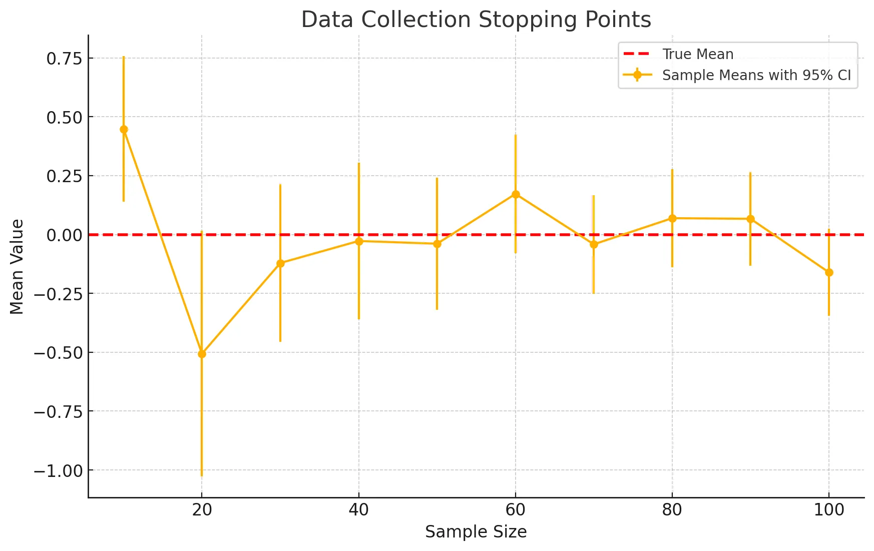
• 샘플 크기에 따른 평균값과 95% 신뢰구간을 나타낸 그래프
• 데이터 수집을 언제 멈출지 결정하는 것은 결과에 영향을 미칠 수 있음
• 이상적으로는 사전에 정해진 계획에 따라야 함

자료수집 중단 시점은 언제 조심해야하는가?

🔥 결과를 이미 정해놓고 그에 맞추기 위해 자료수집을 하고자 할 때

• 50명의 데이터를 수집하기로 했으나, 원하는 결과가 나오지 않자 100명까지 추가로 수집

<예시 코드>

# 데이터 수집 예시
np.random.seed(42)
data = np.random.normal(0, 1, 1000)
sample_sizes = [10, 20, 30, 40, 50, 100, 200, 300, 400, 500]
p_values = []

for size in sample_sizes:
    sample = np.random.choice(data, size)
    _, p_value = stats.ttest_1samp(sample, 0)
    p_values.append(p_value)

# p-값 시각화
plt.plot(sample_sizes, p_values, marker='o')
plt.axhline(y=0.05, color='red', linestyle='dashed', linewidth=1)
plt.title('자료수집 중단 시점에 따른 p-값 변화')
plt.xlabel('샘플 크기')
plt.ylabel('p-값')
plt.show()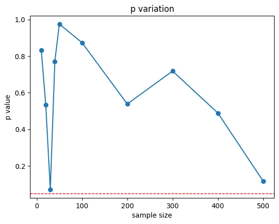

6.5 데이터 탐색과 검증 분리

🫡 검증하기 위한 데이터는 반드시 따로 분리 해놓아야 함!

데이터 탐색과 검증 분리란?

• 데이터 탐색을 통해 가설을 설정하고, 이를 검증하기 위해 별도의 독립된 데이터셋을 사용하는 것
• 이는 데이터 과적합을 방지하고 결과의 신뢰성을 높임
  <예시>
  
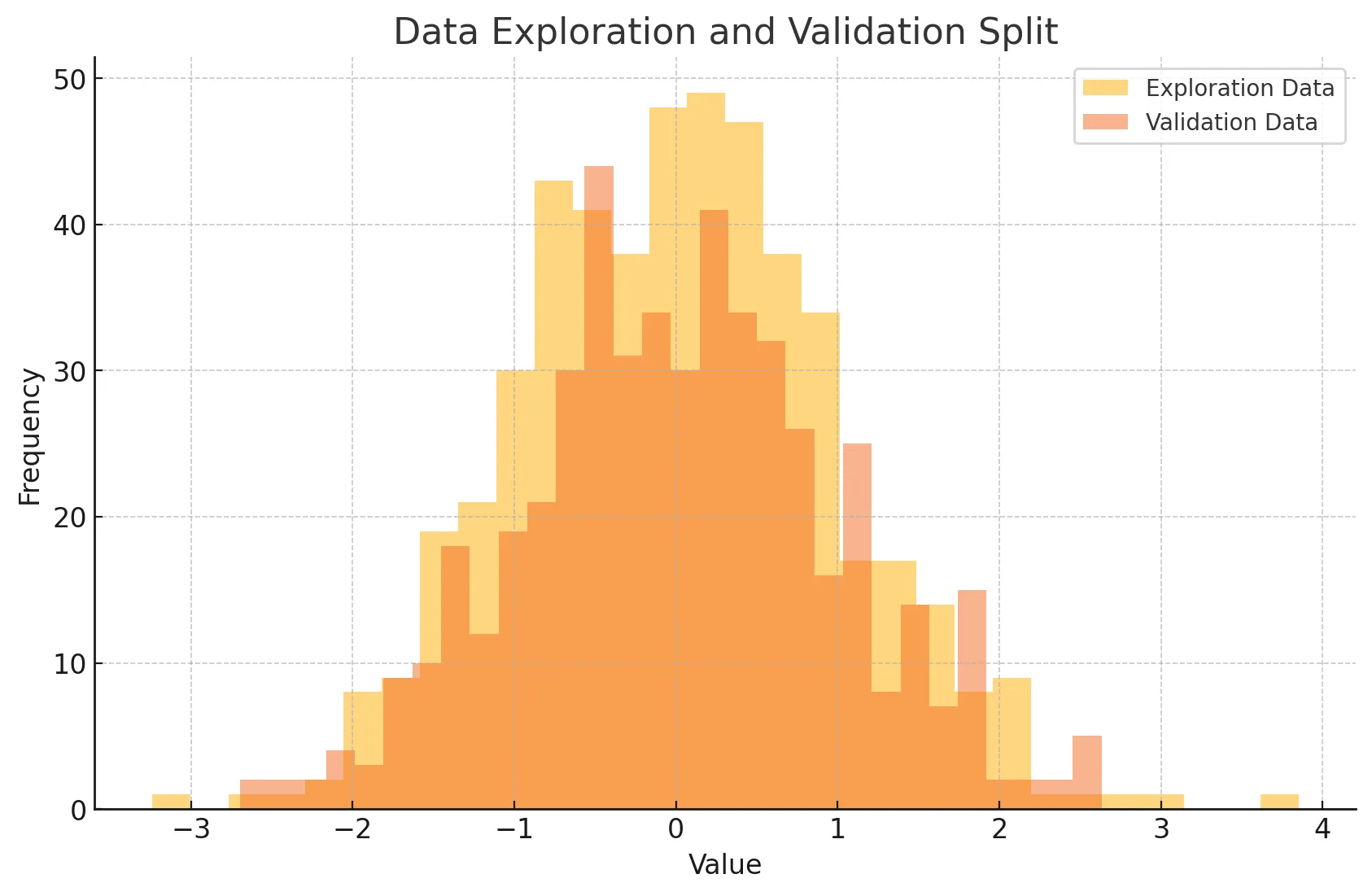
• 탐색 데이터와 검증 데이터를 히스토그램으로 나타냄
• 데이터 탐색과 검증을 분리하면 탐색 과정에서 발견된 패턴이 검증 데이터에서도 유효한지 확인 가능
• 검증 데이터는 철저하게 탐색 데이터와 구분되어져야 함

데이터 탐색과 검증 분리는 언제 사용해야하는가?

👊🏻 검증하기 위한 데이터가 따로 필요할 때

• 데이터셋을 탐색용(training)과 검증용(test)으로 분리하여 사용

<예시 코드>

from sklearn.model_selection import train_test_split

# 데이터 생성
np.random.seed(42)
X = 2 * np.random.rand(100, 1)
y = 4 + 3 * X + np.random.randn(100, 1)

# 데이터 분할 (탐색용 80%, 검증용 20%)
X_train, X_test, y_train, y_test = train_test_split(X, y, test_size=0.2, random_state=42)

# 모델 학습
model = LinearRegression()
model.fit(X_train, y_train)

# 탐색용 데이터로 예측
y_train_pred = model.predict(X_train)

# 검증용 데이터로 예측
y_test_pred = model.predict(X_test)

# 탐색용 데이터 평가
train_mse = mean_squared_error(y_train, y_train_pred)
train_r2 = r2_score(y_train, y_train_pred)
print(f"탐색용 데이터 - MSE: {train_mse}, R2: {train_r2}")

# 검증용 데이터 평가
test_mse = mean_squared_error(y_test, y_test_pred)
test_r2 = r2_score(y_test, y_test_pred)
print(f"검증용 데이터 - MSE: {test_mse}, R2: {test_r2}")