GAN : https://arxiv.org/pdf/1406.2661

0. Abstract

We propose a new framework for estimating generative models via an adversarial process, in which we simultaneously train two models:
a generative model G that captures the data distribution, and a discriminative model D that estimates the probability that a sample came from the training data rather than G

📖 Generative_G 모델은 데이터의 분포를 잡아내고
Discriminative_D 모델은 모델_G에서 나온 것보다 트레이닝된 데이터로부터 표본이 나왔다는 확률을 추정한다.

🤔 "D모델은~ 표본이 나왔다는 확률을 추정한다"라는 말이 무슨 말일까?

👉 D모델이 특정 데이터 샘플이 실제 훈련 데이터에서 온 것인지 아니면 생성된 가짜 데이터에서 온 것인지를 구별하는 확률를 계산한다는 의미..!!

The training procedure for G is to maximize the probability of D making a mistake. This framework corresponds to a minimax two-player game. In the space of arbitrary functions G and D, a unique solution exists, with G recovering the training data distribution and D equal to $\frac{1}{2}$ everywhere

📖 G(생성자)모델의 목표는 D(판별자)가 최대한 실수하게끔 하는 것이고
D모델이 모든 곳에서 $\frac{1}{2}$가 되면 유일한 해답(unique solution) 이 존재하는 것이라고 한다.

🤔 왜 $\frac{1}{2}$ 이 되면 유일한 해답이 존재한다고 하는 것일까?

👉 D모델이 모든 곳에서 $\frac{1}{2}$ 가 되면 G와 D가 최적의 상태에 도달했을 때 G가 생성하는 데이터와 실제 훈련데이터가 구별할 수 없을 정도로 비슷해지기 때문!
D모델은 주어진 데이터가 실제데이터인지 아닌지 판별하는 것이고
G모델은 D모델을 "속여서" 가짜데이터를 실제데이터처럼 보이게 만드는것 -> 따라서 최적의 상태에서는 G가 생성한 데이터가 실제 데이터의 분포와 동일하게 되므로 D는 가짜인지 진짜인지 구별하지 못하므로 $\frac{1}{2}$이 되게 되는것..!

1. Introduction

The promise of deep learning is to discover rich, hierarchical models [2] that represent probability distributions over the kinds of data encountered in artificial intelligence applications, such as natural images, audio waveforms containing speech, and symbols in natural language corpora
(...)
These striking successes have primarily been based on the backpropagation and dropout algorithms, using piecewise linear units [17, 8, 9] which have a particularly well-behaved gradient . Deep generative models have had less of an impact, ①due to the difficulty of approximating many intractable probabilistic computations that arise in maximum likelihood estimation and related strategie, and② due to difficulty of leveraging the benefits of piecewise linear units in the generative context. We propose a new generative model estimation procedure that sidesteps these difficulties.

📖 자연이미지나 waveform 같은 문제는 deeplearning 모델이 잘 적용되었지만, 생성 모델에서는 임팩트가 적었다. 그 이유로는 2가지가 있는데
① MLE(최우도) 관련된 전략에서 발생하는 많은 intractble 한 확률적 계산을 근사화하는 것이 어렵고
② 생성모델 맥락에서 조각별 선형 함수(benefits of piecewise) 의 이점을 활용하는 것이 어렵기 때문이다.

🤔 조각별 선형함수의 이점(leverageing the benefits of piecewise linear units)이 무슨 말??

👉 조각별 선형함수란 신경망에서 자주 사용하는 활성화함수들(ReLU, Softmax,Sigmoid등) 을 말하는 것으로 , 이런 함수들은 경사하강법(gradient descent)를 사용할 때 역전파과정에서 계산이 매우 효율적이다
-> 하지만 생성모델에서는 데이터를 생성하기 위해 복잡한 확률적 계산을 수행해야 하는데 이러한 계산들은 MLE를 사용해도 어려웠다.
->하지만 이 논문에서는 이러한 어려움을 피할 수 있는 새로운 생성 모델 추정 절차를 제안함!!우회(sidestep)

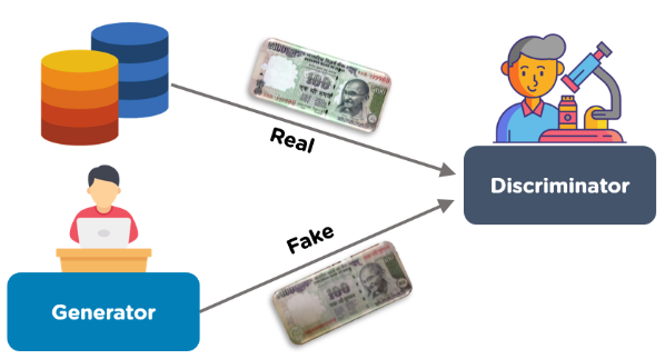
In the proposed adversarial nets framework, the generative model is pitted against an adversary: a discriminative model that learns to determine whether a sample is from the model distribution or the data distribution. The generative model can be thought of as analogous to a team of counterfeiters, trying to produce fake currency and use it without detection, while the discriminative model is analogous to the police, trying to detect the counterfeit currency.
Competition in this game drives both teams to improve their methods until the counterfeits are indistiguishable from the genuine articles.

📖 Adversarial net (적대적신경망)을 제안하는데,
생성자는 위조범, 판별자는 경찰로 서로 경쟁(competition)하는데 결국 진짜와 가짜를 구별할 수 없을 정도로 비슷하게 만든다.

2. Related work

-- 생략--(그전에 나온 모델들에 한계점 설명)

3. Adversarial nets

The adversarial modeling framework is most straightforward to apply when the models are both multilayer perceptrons. To learn the generator’s distribution $p_g$ over data $x$, ①we define a prior on input noise variables $p_z(z)$, then represent a mapping to data space as $G(z; θ_g)$, where $G$ is a differentiable function represented by a multilayer perceptron with parameters $θ_g$. We also define a second multilayer perceptron ②$D(x; θ_d)$ that outputs a single scalar. $D(x)$ represents the probability that $x$ came from the data rather than $p_g$. We train $D$ to maximize the probability of assigning the correct label to both training examples and samples from $G$.

③We simultaneously train $G$ to minimize $log(1 − D(G(z)))$. In other words, $D$ and $G$ play the following two-player minimax game with value function $V (G, D)$:

$\underset G {min} \underset D {max}\ V(D,G) = \mathbb{E}_{x \sim p_{\text{data}}(x)} \left[ \log D(x) \right] + \mathbb{E}_{z \sim p_{z}(z)} \left[ \log \left(1 - D(G(z)) \right) \right]$

매우 중요하므로 꼼꼼히 논문을 읽어보자..!

📖 ① 사전분포 $p_z(z)$ 를 정의하고 이를 데이터를 생성하는 매핑을 $G(z;\theta_g)$로 표현 -> $G$는 매개변수 $\theta_g$로 표현될 수 있는 미분가능한 퍼셉트론(differentiable function)

② 두번째 퍼셉트론$D(x;\theta_d)$로 단일 스칼라 값(single scaler)를 정의하는데 $D(x)$는 $p_g$보다 데이터에서 $x$가 나올 확률 표현

③ 동시에 모델 $G$를 훈련시키는데 $log(1 − D(G(z)))$를 최소화. 그리고 $log \ D(x)$를 최대화.

🤔 읽으면서 3가지 의문점이 들었다.
① 왜 사전분포 $p_z(z)$ 가 필요할까??
② 왜 두번째 퍼셉트론 $D(x;\theta_d)$가 단일 스칼라 값으로 정의되지??
③ 마지막 수식 $\underset G {min} \underset D {max}\ V(D,G) = \mathbb{E}_{x \sim p_{\text{data}}(x)} \left[ \log D(x) \right] + \mathbb{E}_{z \sim p_{z}(z)} \left[ \log \left(1 - D(G(z)) \right) \right]$ 이게 정확히 각각 의미하는 바가 무엇일까??

👉 ① 사전분포(prior distribution)란 모델에서 사용하는 입력 변수에 대한 사전적인 정보나 가정을 표현하는 확률분포이며
$z$는 입력노이즈 변수이고 $p_z(z)$ 는 입력노이즈변수 $z$가 어떤 값일 확률을 정의한다(일반적으로 가우시안임ㅋ{가우시안 없었으면 어쩔뻔했노..})
-> 생성자는 입력노이즈 $z$ 를 기반으로 데이터 샘플을 생성하므로 생성$G$에서 초기 입력값으로 필요함

② $D(x,\theta_d)$가 단일 스칼라값으로 정의되는 이유는 2가지 이다
(1) 이진분류문제이기 떄문에 -> 판별자는 그냥 가짜인지 아닌지 판별하므로

(2) 간단한 출력 해석 -> 단일 스칼라 값으로 출력된 확률 $D(x)$는 데이터가 실제 데이터일 확률을 직관적으로 나타냄!

③ (1) $\underset G {min}\underset D {max}\ V(D,G)$: 생성자$G$는 판별자$D$를 속이기 위해 손실함수를 최소화(min) 하고 판별자$D$는 손실함수를 최대화(max)함

(2) $\mathbb{E}_{x \sim p_{\text{data}}(x)} \left[ \log D(x) \right]$ :실제 데이터에 대한 기대값
-> 실제 데이터$x$ 가 판별자 $D$에 의해 실제 데이터로 올바르게 분류될 확률의 로그

(3) $\mathbb{E}_{z \sim p_{z}(z)} \left[ \log \left(1 - D(G(z)) \right) \right]$ : 생성된 데이터에 대한 기대값
-> 생성된 데이터 $G(x)$가 판별자 $D$ 에 의해 가짜 데이터로 잘못 분류된 확률의 로그 --> 즉, 생성자는 이 값을 최소화할려고 하는 것이고 이는 판별자$D$가 생성된 데이터를 실제 데이터로 잘못 분류하게 만들려고 한다.

In the next section, we present a theoretical analysis of adversarial nets, essentially showing that the training criterion allows one to recover the data generating distribution as $G$ and $D$ are given enough capacity, i.e., in the non-parametric limit.

In practice, we must implement the game using an iterative, numerical approach. Optimizing $D$ to completion in the inner loop of training is computationally prohibitive, and on finite datasets would result in overfitting. Instead, we alternate between k steps of optimizing $D$ and one step of optimizing $G$. This results in $D$ being maintained near its optimal solution, so long as G changes slowly enough. The procedure is formally presented in Algorithm 1.

📖 다음장(4.Theretical Results)에서 이론적 분석을 할 것인데 이 분석은 훈련 기준이 생성자 $G$와 판별자 $D$ 가 충분한 용량을 가질 경우 데이터 생성분포를 회복할 수 있음을 보여줌,,!(4에서 자세히 다룰것.)

판별자 $D$ 를 완벽하게 최적화하는 것은 계산적으로 매우 어려움 => 따라서 $D$를 최적화하는 $k$단계를 반복하고 $G$를 최적화하는 단계를 수행 (다음장에서 Algorithm1으로 자세히 설명예정)

In practice, equation 1 may not provide sufficient gradient for $G$ to learn well. Early in learning, when $G$ is poor, $D$ can reject samples with high confidence because they are clearly different from the training data. In this case, $log(1 − D(G(z)))$ saturates.Rather than training $G$ to minimize $log(1 − D(G(z)))$ we can train G to maximize $log D(G(z))$. This objective function results in the same fixed point of the dynamics of $G$ and $D$ but provides much stronger gradients early in learning.

📖 생성자$G$모델이 부실할 경우에 판별자 $D$가 높은 신뢰도로(high confidence)로 거절할 것이기 때문에, $G$ 모델의 손실함수 $log(1 -D(G(z))$ 를 최소화(min)하는 것보다 $D$모델의 손실함수 $logD(G(z))$ 를 최대화(max) 하는 것이 낫다
-> 이건 뭐 그냥 하나의 꿀팁~🍯(냠냠~)

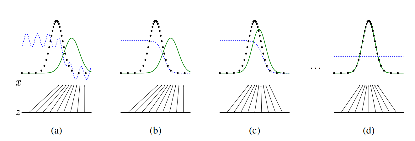
Generative adversarial nets are trained by simultaneously updating the discriminative distribution ($D$, blue, dashed line) so that it discriminates between samples from the data generating distribution (black,dotted line) $p_x$ from those of the generative distribution $p_g$ (G) (green, solid line). The lower horizontal line is the domain from which $z$ is sampled, in this case uniformly. The horizontal line above is part of the domain of $x$. The upward arrows show how the mapping $x = G(z)$ imposes the non-uniform distribution $p_g$ on transformed samples. $G$ contracts in regions of high density and expands in regions of low density of $p_g$.

📖 위 내용에서는 중요한 것이 3가지 있다.
① 파란색 점선은 핀별자(D)이고 ,검은색 점선은 데이터생성분포$p_x$ 이고 초록색 점선은 생성자(G)이다.
② 위쪽으로 나가는 화살표는 매핑 $x = G(x)$ 가 변환된 샘플에 대해 불균일 분포 $p_g$를 부과하는 방법(impose )을 보여준다.
③ 생성자 $G$가 고밀도 영역에서는 수축(contracts)하고 저밀도 영역에서는 팽창(expand)한다.

🤔 솔직히 읽으면서 무슨 소리인가 싶다. 따라서 하나하나 친절하게 따라가보자.

👉 ① 파란색점선은, 판별자로 데이터가 가짜인지 아닌지 판별한다. 초록색실선은, 생성자라는 모델이 만든 가짜 분포이며 검은색점은, 실제 데이터의 분포이다.

②화살표는 생성자(G)가 $z$라는 데이터를 받아서 $x$라는 데이터를 만들어내는지 보여준다. 즉, $G$는 단순하게 데이터를 만드는 것이 아니라 데이터를 특정 패턴에 맞추어서 비균일하게(non-uniformed) 만드는 것이다.

③ 수축 : 생성자가 데이터를 많이 만들어 놓는 곳은 수축(contract)하고 모이게 한다.
팽창 : 생성자가 데이터를 적게 만드는 곳은 팽창(expand) 한다.
-> 즉, 생성자($G$)는 데이터를 만들어내면서, 어디에 모을지(contract) 어디에 퍼뜨릴지(expand)결정함으로써 만들어진 데이터는 원래의 실제 데이터처럼 보이게 할려고 특정 패턴을 따르게 된다.

(a) Consider an adversarial pair near convergence: $p_g$ is similar to $p_{data}$ and $D$ is a partially accurate classifier.

(b) In the inner loop of the algorithm $D$ is trained to discriminate samples from data, converging to $D^∗(x) =\frac{ p_{data}(x)}{p_{data}(x)+p_g(x)}$

(c) After an update to $G$, gradient of $D$ has guided $G(z)$ to flow to regions that are more likely to be classified as data.

(d) After several steps of training, if $G$ and $D$ have enough capacity, they will reach a point at which both cannot improve because $p_g = p_{data}$. The discriminator is unable to differentiate between the two distributions, i.e. $D(x) =\frac{1}{2}$.

📖 (a) 에서 (d)로 가면서 생성자는 실제 데이터의 분포와 가깝게 만들어내면서 판별자는 절반만 맞추는(그러니까 판별하는 의미가 없는) 수준까지 떨어진다. 그게 $D(x) = \frac{1}{2}$ 라고 저자는 말하고 있다.

4. Theretical Results

---

Algorithm1이 여기 논문에서는 매우 중요하다!!! 따라서 자세히 세부적으로 구석구석 핥아보자.(근데 그냥 역전파라서 볼거는 별루 없음ㅋ)

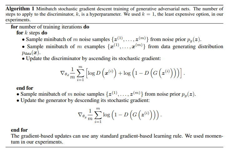
📖 ① 판별자(D) 훈련
$k$ step 동안
$1)$ 사전노이즈분포 $p_g(z)$ 에서 $m$개의 노이즈 샘플 추출함.
$2)$ 참분포 $p_{data}(x)$에서 $m$개의 데이터 추출함.
$3)$ 그 다음에 판별자를 확률적 경사하강법으로 업데이트함

② 생성자(G) 훈련
$1)$ 사전노이즈 분포$p_g(z)$ 에서 $m$개의 샘플 뽑고
$2)$ 이것도 동일하게 확률적경사하강법 수행.

..
참쉽죠?(아마 저자도 생각보다 별거 없는 거라고 알고리즘1이라고 대충 지은듯)

---

The generator $G$ implicitly defines a probability distribution $p_g$ as the distribution of the samples $G(z)$ obtained when $z ∼ p_z$. Therefore, we would like Algorithm 1 to converge to a good estimator of $p_{data}$, if given enough capacity and training time. The results of this section are done in a nonparametric setting, e.g. we represent a model with infinite capacity by studying convergence in the space of probability density functions. We will show in section 4.1 that this minimax game has a global optimum for $p_g = p_{data}$. We will then show in section 4.2 that Algorithm 1 optimizes Eq 1, thus obtaining the desired result

📖 우리는 Algorithm1이 충분한 용량(capacity)과 훈련시간(time)을 제공받았을때 $p_{data}$를 좋은 추정치(good estimator)가 되기를 바라고, 섹션4.1 에서 미니맥스 게임이 $p_g = p_{data}$ 일때 전역최적해(global optimum)을 가진것을 보여줄 것이고 , 섹션4.2에서 Algorithm1이 식1을 최적화하여 원하는 결과를 얻는 다는 것을 증명.

👉 ① Algorithm1이 좋은 모델이라면 $p_g \simeq p_{data}$으로 훈련되길 기대.좋은 추정치(여기서 좋은 추정치란, 생성된 데이터분포 $p_g$가 실제 데이터분포 $p_{data}$ 와 매우 근접한 상태)

② 미니맥스 게임(GAN에서 생성자와 판별자간의 게임) 이 $p_g =p_{data}$일때 전역해를 가진다는 것이고,이는 생성자가 완벽히 훈련되면 생성된 데이터 분포가 실제 데이터 분포와 일치하게 된다는 것을 의미함.(내말이 맞음을 섹션 4.1에서 증명)

③ Algorithm1이 특정방정식(eq1)에 가까워지면(optimize) 원하는 결과를 얻는다는 것을 섹션4.2에서 보여줌

4.1 Global Optimality of $p_g = p_\text{data}$

We first consider the optimal discriminator $D$ for any given generator $G$.
Proposition 1. For $G$ fixed, the optimal discriminator $D$ is
$D_{G}^*{(x)} = \frac{p_{data}(x)}{p_{data}(x) + p_g(x)}$

증명은 논문참조

Theorem 1. The global minimum of the virtual training criterion $C(G)$ is achieved if and only if $p_g = p_{data}$. At that point, $C(G)$ achieves the value − $log 4$.

증명은 논문참조

4.2 Convergence of Algorithm1

Proposition 2. If $G$ and $D$ have enough capacity, and at each step of Algorithm 1, the discriminator is allowed to reach its optimum given $G$, and $p_g$ is updated so as to improve the criterion

$\mathbb{E}_{x \sim p_{data}} \left[ \log D^*_G(x) \right] + \mathbb{E}_{x \sim p_g} \left[ \log \left(1 - D^*_G(x)\right) \right]$ converges to $p_{data}$

증명은 논문참조.

5. Experiment

-생략

6. Advantages and disadvantages

The disadvantages are primarily that there is no explicit representation of $p_g(x)$, and that $D$ must be synchronized well with $G$ during training (in particular, $G$ must not be trained too much without updating $D$, in order to avoid $“the\ Helvetica\ scenario”$ in which $G$ collapses too many values of $z$ to the same value of $x$ to have enough diversity to model $p_{data}$), much as the negative chains of a Boltzmann machine must be kept up to date between learning step

📖 단점은 3가지
① $p_g{(x)}$ 가 명시적으로 표현하지 않고
② 생성자$G$과 판별자 $D$가 동기화가 잘 되어야함 -> 이는 train시키는데 상당히 어려움을 겪음
③ 생성자가 너무 많은 값을 동일하게 매핑해서 데이터의 다양성을 잃어버릴 수 있음.

The advantages are that Markov chains are never needed, only backprop is used to obtain gradients, no inference is needed during learning, and a wide variety of functions can be incorporated into the model(...)

The aforementioned advantages are primarily computational. Adversarial models may also gain some statistical advantage from the generator network not being updated directly with data examples, but only with gradients flowing through the discriminator. This means that components of the input are not copied directly into the generator’s parameters. Another advantage of adversarial networks is that they can represent very sharp, even degenerate distributions, while methods based on
Markov chains require that the distribution be somewhat blurry in order for the chains to be able to mix between modes

📖장점
① 마르코브 체인을 안 써도 됨 -> 오직 역전파 알고리즘 사용!
② 추론불필요 -> 오직 판별자(D)에서 얻음 기울기만 사용
③ 컴퓨팅자원 많이 줄임.

7. Conclusions and future work

1. A conditional generative model $p(x | c)$can be obtained by adding $c$ as input to both $G$ and $D$.

2. Learned approximate inference can be performed by training an auxiliary network to predict $z$ given $x$. This is similar to the inference net trained by the wake-sleep algorithm [15] but with the advantage that the inference net may be trained for a fixed generator net after the generator net has finished training.

3. One can approximately model all conditionals $p(xS | x=/S)$ where S is a subset of the indices
   of x by training a family of conditional models that share parameters. Essentially, one can use
   adversarial nets to implement a stochastic extension of the deterministic MP-DBM [11].

4. Semi-supervised learning: features from the discriminator or inference net could improve performance of classifiers when limited labeled data is available.

5. Efficiency improvements: training could be accelerated greatly by divising better methods for coordinating $G$ and $D$ or determining better distributions to sample $z$ from during training.

8. Code 구현

(나중에... )