🐍 오래된 논문이니까 간단하게만 리뷰하고 마치겠다.

• VGG:https://arxiv.org/abs/1409.1556

VGG_(Visual Geometry Group)

0. Abstract

In this work we investigate the effect of the convolutional network depth on its accuracy in the large-scale image recognition setting. Our main contribution is a thorough evaluation of networks of increasing depth using an architecture with very small (3×3) convolution filters, which shows that a significant improvement on the prior-art configurations can be achieved by pushing the depth to 16–19 weight layers. These findings were the basis of our ImageNet Challenge 2014 submission, where our team secured the first and the second places in the localisation and classification tracks respectively. We also show that our representations generalise well to other datasets, where they achieve state-of-the-art results. We have made our two best-performing ConvNet models publicly available to facilitate further research on the use of deep visual representations in computer vision.

📖 저자들이 VGG_Net 으로 하는 기여는, 매우 작은 (3x3) convolutional filter 를 사용하는 것인데 이것은 가중치 레이어의 깊이를 16-19층으로 확장함으로써 개선 상당한 개선(significant improvement)했다고 함.

1. Introduction

(...)As a result, we come up with significantly more accurate ConvNet architectures, which not only achieve the state-of-the-art accuracy on ILSVRC classification and localisation tasks, but are also applicable to other image recognition datasets, where they achieve excellent performance even when used as a part of a relatively simple pipelines (...)

📖 더 정확한 ConvNet Architecture 제안.

2. ConvNet Configuration

2.1 Architecture

During training, the input to our ConvNets is a fixed-size 224 × 224 RGB image. The only preprocessing we do is subtracting the mean RGB value, computed on the training set, from each pixel.① The image is passed through a stack of convolutional (conv.) layers, where we use filters with a very small receptive field: 3 × 3 (which is the smallest size to capture the notion of left/right, up/down, center). In one of the configurations we also utilise

② 1 × 1 convolution filters, which can be seen as a linear transformation of the input channels (followed by non-linearity). The convolution stride is fixed to 1 pixel; the spatial padding of conv. layer input is such that the spatial resolution is preserved after convolution, i.e. the padding is 1 pixel for 3 × 3 conv. layers.

③Spatial pooling is carried out by five max-pooling layers, which follow some of the conv. layers (not all the conv. layers are followed by max-pooling). Max-pooling is performed over a 2 × 2 pixel window, with stride 2. A stack of convolutional layers (which has a different depth in different architectures) is followed by three Fully-Connected (FC) layers: the first two have 4096 channels each, the third performs 1000-way ILSVRC classification and thus contains 1000 channels (one for each class). The final layer is the soft-max layer. The configuration of the fully connected layers is the same in all networks.

④All hidden layers are equipped with the rectification (ReLU (Krizhevsky et al., 2012)) non-linearity. We note that none of our networks (except for one) contain Local Response Normalisation
(LRN) normalisation (Krizhevsky et al., 2012): as will be shown in Sect. 4, such normalisation does not improve the performance on the ILSVRC dataset, but leads to increased memory consumption and computation time. Where applicable, the parameters for the LRN layer are those of (Krizhevsky et al., 2012).

📖 VGG 특징요약해보면 이렇다
① 매우작은(3x3크기)의 필터를 사용
-> 이미지를 처리할 때 3x3필터를 사용하여 특징 추출

② 1x1크기의 합성곱 필터는 입력 채널에 대한 선형 변환으로 볼 수 있다.

③ 공간 풀링(spatial pooling)은 다섯 개의 맥스풀링(max-pooling) 계층에 의해서 수행

④ 모든 은닉층은 ReLU 라는 비선형 활성화 함수로 작용.

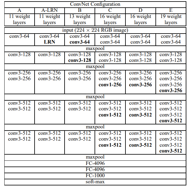
2.2 Configuration

All configurations follow the generic design presented in Sect. 2.1, and differ only in the depth: from 11 weight layers in the network A (8 conv. and 3 FC layers) to 19 weight layers in the network E (16 conv. and 3 FC layers).

we report the number of parameters for each configuration. In spite of a large depth, the number of weights in our nets is not greater than the number of weights in a more shallow net with larger conv. layer widths and receptive fields (144M weights in (Sermanet et al., 2014))

📖 깊은 층임에도 불구하고, 전체 가중치의 수는 얕은 네트워크의 가중치 수보다 많지는 않다.

👉 즉, 작은 필터와 적절한 채널 수를 사용하면서 깊이를 증가시켰기 때문에, 네트워크의 복잡성을 효율적으로 관리하면서도 성능을 유지하거나 개선할 수 있음을 강조하고 있음!

2.3 DISCUSSION

we use very small $3 × 3$ receptive fields throughout the whole net,which are convolved with the input at every pixel (with stride 1) . It is easy to see that a stack of two 3×3 conv. layers (without spatial pooling in between) has an effective receptive field of $5×5$.three such layers have a $7 × 7$ effective receptive field.

📖 (~번역이 더럽게 어렵다) 두 개의 $3 ×3$ 컨볼루션 레이어를 쌓으면 수용필드(receptive field)는 $5 ×5$ 가 되고, 세개의 레이어를 쌓으면 $7 ×7$필드가 된다.

So what have we gained by using, for instance, a stack of three $3×3$ conv. layers instead of a single $7×7$ layer?

First, ① we incorporate three non-linear rectification layers instead of a single one, which makes the decision function more discriminative

Second, ② we decrease the number of parameters: assuming that both the input and the output of a three-layer $3 × 3$ convolution stack has C channels, the stack is parametrised by $3$ ($3^2C^2$) = $27C^2$ weights; at the same time, a single 7 × 7 conv. layer would require $7^2C^2 = 49C^2$ parameters, i.e. 81% more. This can be seen as imposing a regularisation on the $7 × 7$ conv. filters, forcing them to have a decomposition through the $3 × 3$ filter

📖 왜 $3 × 3$ 필터를 쓰는가?
첫번째, 하나의 $7 × 7$ 레이어 대신 3개의 비선형 정규화 레이어를 사용함으로써 더 좋은(disciminative) 결정함수(decision function)이 만들어짐

둘째로, 파라미터 수를 줄일 수 있음
예를 들어 인풋과 아웃풋이 $3×3$ 이고 convolution 이고 $C$채널이라면 27 개 파라미터 인데
$7×7$이라면 $49$다. 이는 27개보다 81% 많은 파라미터수를 요구하는 것이고(7x7필터에 규제를 가하는 것) 필터가 $3×3$ 로 강제로(forcing) 분해(decomposition)하는 것.

3.CLASSIFICATION FRAMEWORK

• 이후 모두 생략함. 자세한건 논문 참조.

---

ResNet(Residual Network)

• ResNet: https://arxiv.org/abs/1512.03385

0. Abstract

Deeper neural networks are more difficult to train. We present a residual learning framework to ease the training of networks that are substantially deeper than those used previously. We explicitly reformulate the layers as learning residual functions with reference to the layer inputs, instead of learning unreferenced functions. We provide comprehensive empirical evidence showing that these residual networks are easier to optimize, and can gain accuracy from considerably increased depth(..)The depth of representations is of central importance for many visual recognition tasks. Solely due to our extremely deep representations, we obtain a 28% relative improvement on the COCO object detection dataset(...)

📖 잔차학습을 제안하는데 이전에 사용한 네트워크 모델보다 더 깊은 네트워크를 학습하는 과정을 쉽게 하기 위해 잔차학습 프레임 워크를 제안한다.

👉이 논문에서 잔차학습(residual learning)이 나온다. 이는 반드시 알아야 하는 개념이다. 왜냐하면 잊을만 하면 나오는 architecture 이기 때문이다.

1. Introduction

(...) When deeper networks are able to start converging, a
degradation problem has been exposed: with the network
depth increasing, accuracy gets saturated (which might be
unsurprising) and then degrades rapidly. Unexpectedly,
such degradation is not caused by overfitting, and adding
more layers to a suitably deep model leads to higher training error, as reported in [11, 42] and thoroughly verified by our experiments. Fig. 1 shows a typical example.

There exists a solution by "construction" to the deeper model: the added layers are identity mapping, and the other layers are copied from the learned shallower model. The existence of this constructed solution indicates that a deeper model should produce no higher training error than its shallower counterpart. But experiments show that our current solvers on hand are unable to find solutions thaare comparably good or better than the constructed solution (or unable to do so in feasible time).

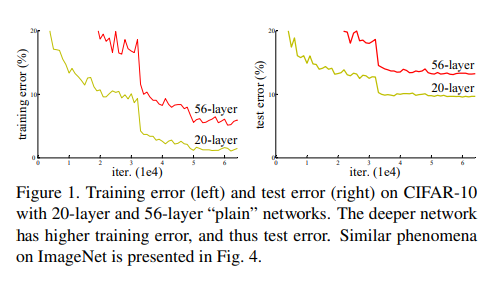
📖 깊은 네트워크에 갈 수록 수렴(converging)하지만, 성능저하(degradation)문제가 생긴다.(생략) 하지만 깊은 모델에서도 해답(solution)이 "구성적"(construction)으로 존재한다. 추가된 레이어들은 정체성매핑(identity mapping) 을 하며 다른 레이어들은 학습된 더 얕은 모델에서 복사된다..!
-> 구성적 솔루션이 존재한다는 의미는 더 깊은 모델일수록 더 높은 훈련 오류를 낼 이유가 없다 것을 의미

👉 그러니까 기존에는 모델이 깊어질수록 훈련 오류가 있었는데, 이론적으로는 이게 해결이 가능했는데, 경험상(experiment) 솔루션을 찾을 수 없었다.

In this paper, we address the degradation problem by introducing a deep residual learning framework. Instead of hoping each few stacked layers directly fit a desired underlying mapping, we explicitly let these layers fit a residual mapping. Formally, denoting the desired underlying mapping as $\mathcal H(x)$, we let the stacked nonlinear layers fit another mapping of $\mathcal F(x) := \mathcal H(x)−x$. The original mapping is recast into $\mathcal F(x)+x$. We hypothesize that it is easier to optimize the residual mapping than to optimize the original, unreferenced mapping. To the extreme, if an identity mapping were optimal, it would be easier to push the residual to zero than to fit an identity mapping by a stack of nonlinear layers.

📖 깊은 잔차 학습 프레임워크(deep residual learning framework)를 제안한다. 몇 개의 쌓인 레이어들이(stacked layers) 원하는 매핑을 직접 맞추도록 하는 대신에, 이 레이어들이 잔차매핑(residual mapping)을 학습하도록 명시적으로 설정함.

우리가 원하는 매핑을 $\mathcal H(x)$라고 하고 쌓인 비선형 레이어들이 다른 매핑인 $\mathcal F(x) := \mathcal H(x) -x$를 학습하도록 한다. 따라서 원래 매핑 $\mathcal H(x)$는 $\mathcal F(x) +x$로 재구성되고 잔차 매핑을 최적화하는 것이 쉽다고 가정

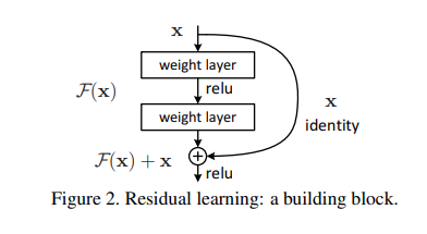
The formulation of $\mathcal F(x) +x$ can be realized by feedforward neural networks with “shortcut connections” (Fig. 2). Shortcut connections [2, 34, 49] are those skipping one or more layers. In our case, the shortcut connections simply perform identity mapping, and their outputs are added to the outputs of the stacked layers (Fig. 2). Identity shortcut connections add neither extra parameter nor computational complexity. The entire network can still be trained end-to-end by SGD with backpropagation

📖 $\mathcal H(x) = \mathcal F(x) +x$의 형식은 스킵연결(short connection)을 사용하는 피드포워드 방식임. 그리고 전체적인 네트워크는 SGD 역전파를 통해 end-to-end.로 훈련(train)될 수 있음!

2. Related Work

-생략!

3. Deep Residual Learning

3.1 Residual Learning

Let us consider $\mathcal H(x)$ as an underlying mapping to be fit by a few stacked layers (not necessarily the entire net),with $x$ denoting the inputs to the first of these layers. If one hypothesizes that multiple nonlinear layers can asymptotically approximate complicated functions, then it is equivalent to hypothesize that they can asymptotically approximate the residual functions, i.e., $\mathcal H(x) − x$ (assuming that the input and output are of the same dimensions). So rather than expect stacked layers to approximate $\mathcal H(x)$, we explicitly let these layers approximate a residual function $\mathcal F(x) := H(x) − x$. The original function thus becomes $\mathcal F(x)+x$. Although both forms should be able to asymptotically approximate the desired functions (as hypothesized), the ease of learning might be different

📖 ① 만걍 여러 비선형 레이어가 복잡한 함수들을 점근적으로(asymptotically) 근사할 수 있다고 가정한다면, 이는 비선형 레이어들이 잔차함수 $\mathcal H(x) -x$를 점근적으로 근사할 수 있다고 가정한 것과 같음.

② $\mathcal H(x)$ 라는 원래의 매핑을 근사하도록 하는 것보다 -> $\mathcal F(x) := H(x) − x$라는 잔차함수를 근사하도록함.

🤔 왜 잔차함수를 근사하도록 함??

👉 대가정을 비선형 레이어들이 복잡한 함수를 점근적으로 가까워지게 한다고 하면, 이와 동일하게 $\mathcal H(x) -x$라는 잔차함수를 근사할 수 있다고 볼 수 있는 것임.

3.2 Identity Mapping by Shortcuts

We adopt residual learning to every few stacked layers. A building block is shown in Fig. 2. Formally, in this paper we consider a building block defined as:

$y = \mathcal F(x, {W_i}) + x$ -> Eqn(1)

Here $x$ and $y$ are the input and output vectors of the layers considered. The function $\mathcal F(x, {W_i})$represents the residual mapping to be learned.For the example in Fig. 2 that has two layers, $\mathcal F = W_2σ(W_1x)$ in which σ denotes $ReLU$ and the biases are omitted for simplifying notations. The operation $\mathcal F + x$ is performed by a shortcut connection and element-wise addition. We adopt the second nonlinearity after the addition.
(...)The dimensions of $x$ and $\mathcal F$ must be equal in Eqn.(1). If this is not the case (e.g., when changing the input/output channels), we can perform a linear projection $W_s$ by the shortcut connections to match the dimensions:

$y = \mathcal F(x, {W_i}) + W_sx$.

📖 $y = \mathcal F(x, {W_i}) + x$ <- 이 식이 핵심이다.
①$\mathcal F(x, {W_i})$ : 잔차 함수이며 입력 $x$에 가중치 $W_i$를 적용해야 하는 잔차 매핑.-> 구체적으로는 여러 층(layer)으로 이루어진 네트워크에서 각 층의 가중치와 활성화 함수(예: ReLU)를 사용해 입력값을 변환하는 과정을 의미

② $x$ : 입력값 -> 이 부분이 지름길연결(shortcut connection) 또는 스킵연결이라고 불림.

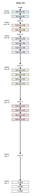
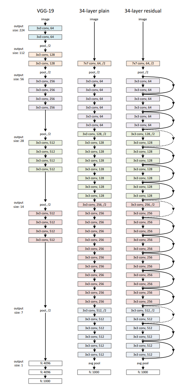
3.3 Network Architectures

Left : VGG_net
Middle : plain
Right : ResidualNet

3.4 Implementation