[ML] tensorflow 몸무게로 키 예측해보기

라이브러리 불러오기

from tensorflow.keras.models import Sequential
from tensorflow.keras.layers import Dense
import numpy as np
from sklearn.preprocessing import StandardScaler
from sklearn.model_selection import train_test_split
from sklearn.metrics import mean_squared_error

키와 몸무게 데이터

weights = np.array([87,81,82,92,90,61,86,66,69,69,76,53,70])
heights = np.array([187,174,179,192,188,160,179,168,168,174,182,162,176])

데이터 스케일링

scaler = StandardScaler()
weights_scaled = scaler.fit_transform(weights.reshape(-1,1))
heights_scaled = scaler.fit_transform(heights.reshape(-1,1))

데이터 분리

X_train, X_test, y_train, y_test = train_test_split(weights_scaled,
heights_scaled, test_size=0.2, random_state=42)

모델1 : 단일 레이어 아키텍쳐

model = Sequential()
dense_layer = Dense(units=1, input_shape=[1])
model.add(dense_layer)
model.compile(optimizer='adam',loss='mean_squared_error')
model.summary()

error : UserWarning: Do not pass an input_shape/input_dim argument to a layer. When using Sequential models, prefer using an Input(shape) object as the first layer in the model instead.

이 메시지는 TensorFlow/Keras가 Sequential 모델의 권장 사용법을 나타낸다.
현재 코드도 작동은 하지만, Input 객체를 사용하는 방식이 명확하고 유지보수하기 좋으니 오류 메세지가 나오는 것.

Dense,Input 라이브러리 추가 import

from tensorflow.keras.layers import Dense, Input

(수정) 모델1 : 단일 레이어 아키텍쳐

# 모델 정의
model = Sequential([
    Input(shape=(1,)),  # Input 객체를 사용
    Dense(units=1)      # 이후 레이어 정의
])

모델에서 Sequential Input으로 shape을 다시 지정해주었다.

model.summary()

model.compile(optimizer='adam', loss='mean_squared_error')
model.summary()

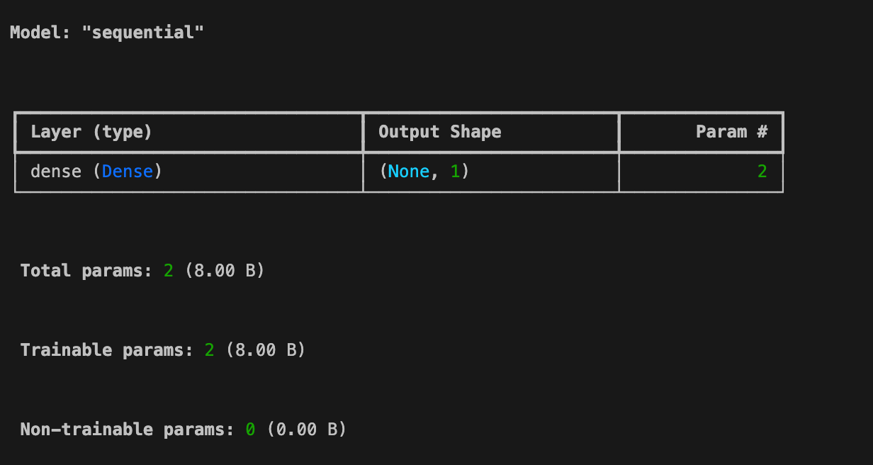
Param : 2 라는 건 (가중치 하나 + 바이어스 하나 = 총 두개) 라는 얘기다.

model.fit()

model.fit(X_train, y_train, epochs=100, verbose=0)

verbose=0은 fit 메서드에서 사용되고 모델 학습 중 출력되는 로그의 상세 정도를 설정하는 옵션

verbose=0:

• 아무런 로그를 출력하지 않는다
• 학습 상태를 확인하지 않아도 될 때 유용

verbose=1 (기본값):

• 학습 진행 상황을 한 줄씩 출력
• epoch별로 손실 값을 표시하며, 진행 바(progress bar)가 표시

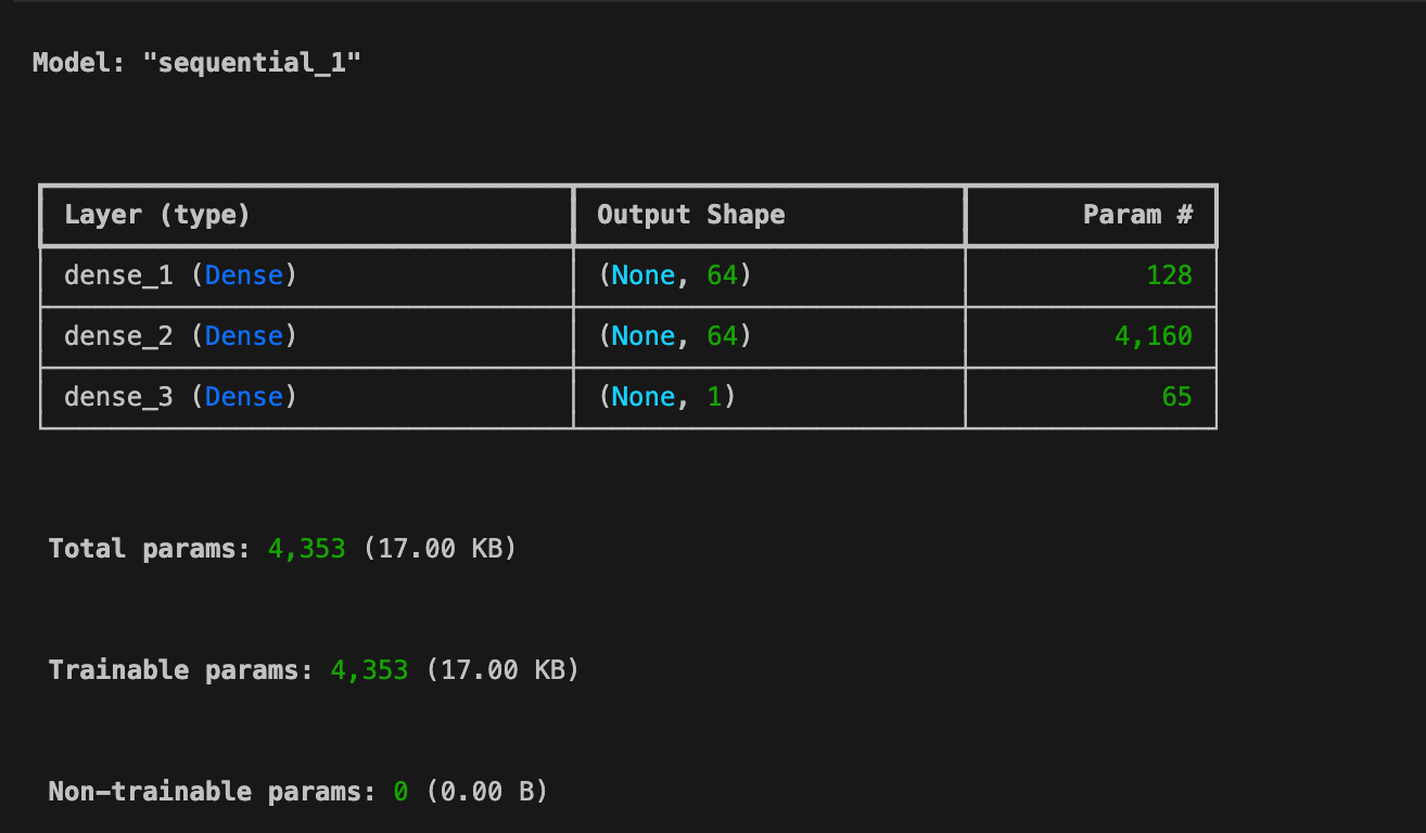
모델2 : Hidden Layer 아키텍쳐

model2 = Sequential([
    Input(shape=(1,)),
    Dense(units=64, activation='relu'),
    Dense(units=64, activation='relu'),
    Dense(units=1)
])

model2.summary()

model2.compile(optimizer= 'adam',loss= 'mean_squared_error')
model2.summary()
model2.fit(X_train, y_train, epochs=150, verbose=0)

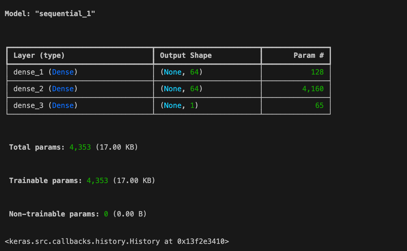
model2.summary(), model2.fit() 의 결과가 한꺼번에 나온 모습.

예측 및 평가

predictions = model.predict(X_test)
predictions2 = model2.predict(X_test)

mse_model1 = mean_squared_error(y_test, predictions)
mse_model2 = mean_squared_error(y_test, predictions2)

print(f"Model 1 MSE: {mse_model1}")
print(f"Model 2 MSE: {mse_model2}")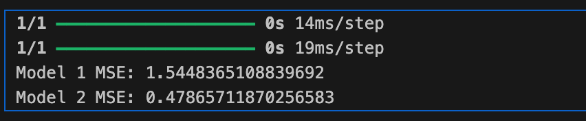

스케일링 후 Model 2의 MSE가 낮아진 것은 긍정적인 결과다.

은닉층이 있는 복잡한 모델에서는 스케일링된 데이터를 사용하면 좋은 성능을 얻을 가능성이 크다

값 예측 Test

def predict_height(weight):
    # 입력 데이터를 2D 배열로 변환
    weight_array = np.array([[weight]])
    # 스케일링 적용
    weight_scaled = scaler.transform(weight_array)
    # 예측
    height_scaled = model2.predict(weight_scaled)
    # 스케일 복원
    height_original = scaler.inverse_transform(height_scaled)
    # 결과 출력
    return f"predict({weight}) = {height_original[0, 0]:.2f}"
# 결과
result = predict_height(90)
print(result)

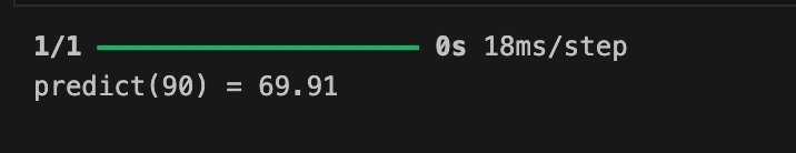
!!!? 결과 값이 이상하게 나왔다.
보통 몸무게가 90일 경우, 키가 최소 170은 넘어줘야 할 것 같은데, 전혀 이상한 값이 나왔다.

어디서 잘못된 것일까

지금처럼 이상한 값이 나왔을 경우 예상해 볼 수 있는 문제로는

1. StandardScaler의 스케일링 문제
2. 모델의 학습 및 예측 문제
3. 모델 성능 문제
4. 스케일링 후 복원 문제

등을 생각해 볼 수 있었는데

코드를 처음부터 둘러보니 StandardScaler의 문제였다.
키와 몸무게는 같은 단위를 사용하지 않기 때문에 각자 다른 스케일러를 사용해줘야 하고, 그에 맞게 코드를 수정해 주었다.

데이터 스케일링 수정

weight_scaler = StandardScaler()
height_scaler = StandardScaler()
weights_scaled = weight_scaler.fit_transform(weights.reshape(-1,1))
heights_scaled = height_scaler.fit_transform(heights.reshape(-1,1))

값 예측 Test 수정

def predict_height(weight):
    # 입력 데이터를 2D 배열로 변환
    weight_array = np.array([[weight]])
    # 스케일링 적용
    weight_scaled = weight_scaler.transform(weight_array)
    # 예측
    height_scaled = model2.predict(weight_scaled)
    # 스케일 복원
    height_original = height_scaler.inverse_transform(height_scaled)
    # 결과 출력
    return f"predict({weight}) = {height_original[0, 0]:.2f}"
# 예측
result = predict_height(90)
print(result)

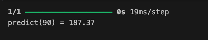
이렇게 예측 결과가 잘 나오는 모습.