cifar10 데이터 셋을 이용한 과제중 alexNet을 이용한 과제가 있었는데 alexNet구조를 다시 볼겸 파인튜닝이 가능할런지 볼 겸 간단하게 시간때우기 겸 진행해 보았습니다.
가장 기본적인 구조로 진행한 것은 다음과 같습니다.
CNN의 대표적인 모델이고,
AlexNet은 인공지능의 Classification 대회인 ILSVRC에서 2012년에 당시 오차율 16.4%로 다른 모델들을 압도하고 우승한 모델입니다. 지금 이 수치를 보자면 그렇게 좋은 정확도가 아니지만, 저 당시에는 굉장한 정확도였다고 합니다. 그도 그럴 것이 2011년에 우승했던 모델의 오차율이 25.8%였으니, 오차율로만 보자면 성능이 40% 만큼 좋아진 셈입니다. AlexNet의 'Alex'는 모델 논문의 저자인 Alex Khrizevsky의 이름을 딴 것이라고 합니다.
AlexNet의 구조
AlexNet은 총 8개의 층으로 구성되어 있습니다. 첫 5개 층은 Convolution, 그 뒤 3개 층은 Fully-Connected 층입니다. 각각의 층들은 하나의 이미지에 대해 독립적으로 특징을 추출하여(Feature Extraction) 가중치를 조정함으로써 필터를 학습시킵니다. 층별로 어떤 역할을 하는지 살펴보겠습니다.
1,2 layer은 Max Pooling 층입니다. 이를 통해 데이터의 중요한 요소들만 요약하여 추출합니다.
3,4,5 layer은 서로 직접 연결되는 형태로 이루어져 있습니다.
5 layer 뒤에는 Max Pooling을 통해 Fully Connected 층 두 개로 구성됩니다. 1~5 layer에서 학습된 데이터들은 Fully Connected 층에서 분류됩니다.
6~7층은 dense와 dropout을 거쳐서 최종적으로는 Softmax 분류기로 분류됩니다.
AlexNet의 구조적 특징들로 Non-overlapping pooling과 Overlapping pooling 비교하면
Overlapping Pooling Layer는 다른 CNN 모델에서 Pooling은 일반적으로 필터를 겹치지 않게 Stride를 적절히 조정하여 사용합니다. 그러나 AlexNet에서는 Stride를 좁혀 Overlapping 하는 구조를 만들었습니다. 이 경우, 정확도는 약 0.4%가 향상되지만 Overlapping의 사용은 연상량을 증가시켰습니다.
그 외에 Data Augmentation, gpu사용을 통한 병렬 계산 등 다양한 방법으로 보다 나은 성능을 얻어냈습니다.
현재로서는 보편화된 기법들이라고 볼 수 있으나 발표당시에는 꽤나 생소한 개념을 사용한 기법이었던 것을 알 수 있습니다.
기본적인 alexNet을 이용한 과제내용(코드내용)은 다음과 같습니다.
# Load Libraries (set the gpu available)
import numpy as np
import tensorflow as tf
import tensorflow_datasets as tfds
import matplotlib.pyplot as plt

gpus = tf.config.list_physical_devices('GPU')
print("Num GPUs Available: ", len(gpus))
# Prepare Datasets
dataset = 'cifar10'

if dataset == 'cifar10':
    # Load the original CIFAR10 dataset
    # CIFAR10 dataset contains 50000 training images and 10000 test images of 32x32x3 pixels
    # Each image contains a small object such as bird, truck, etc...
    (ds_train, ds_test, ds_val), ds_info = tfds.load('cifar10', split=['train[:80%]', 'test', 'train[80%:]'],
                                                 batch_size=None, shuffle_files=True, as_supervised=True,
                                                 with_info=True)
elif dataset == 'imagenette':
    # Imagenette is a subset of 10 easily classified classes from Imagenet
    # (tench, English springer, cassette player, chain saw, church, French horn, garbage truck, gas pump, golf ball, parachute).
    (ds_train, ds_test, ds_val), ds_info = tfds.load('imagenette/320px-v2', split=['train', 'validation[:50%]', 'validation[50%:]'],
                                                 batch_size=None, shuffle_files=True, as_supervised=True,
                                                 with_info=True)
else:
    print('Dataset Error')

print(ds_info.features)
print(ds_info.splits)
print(ds_info.splits['train'].num_examples)

# classify the classes in the dataset
n_channels = ds_info.features['image'].shape[-1]

if dataset == 'imagenette':
    classes = ['tench', 'English springer', 'cassette player', 'chain saw',
               'church', 'French horn', 'garbage truck', 'gas pump',
               'golf ball', 'parachute']
else:
    classes = ds_info.features['label'].names
n_classes = ds_info.features['label'].num_classes
# sort the dataset into trian,valid and test
n_train = len(ds_train)
n_test = len(ds_test)
n_val = len(ds_val)

print(n_train,n_test,n_val)
# Show a Simple Data
idx = np.random.randint(n_train-1)

for element in ds_train.skip(idx).take(1):
    image, label = element

print('Image demension:', image.shape, ', label:',label.numpy())

dimage = tf.reshape(image, image.shape)
plt.matshow(dimage)
plt.show()
print('The picture is', classes[label]) # print the prediction
# Building Input Data pipelines
def tfds_4_NET(image, label):

    image = tf.image.resize((image / 255), [227,227], method='bilinear')  # normalization the image
    label = tf.one_hot(label, n_classes)   # one-hot encoding

    return image, label
n_batch = 64  # set the number of batches
# set the feature maps
dataset = ds_train.map(tfds_4_NET, num_parallel_calls=tf.data.AUTOTUNE)
dataset = dataset.shuffle(buffer_size = 256).batch(batch_size=n_batch)

valiset = ds_val.map(tfds_4_NET, num_parallel_calls=tf.data.AUTOTUNE)
valiset = valiset.shuffle(buffer_size = 256).batch(batch_size=n_batch)

testset = ds_test.map(tfds_4_NET, num_parallel_calls=tf.data.AUTOTUNE)
testset = testset.shuffle(buffer_size = 256).batch(batch_size=n_batch)
# Define the network of AlexNet with Keras Sequential API
import tensorflow as tf

# Define the AlexNet model in TensorFlow/Keras
AlexNet = tf.keras.Sequential([
    # Layer 1
    tf.keras.layers.Conv2D(96, (11, 11), strides=(4, 4), activation='relu', input_shape=(227, 227, 3)), # convolution2D (1st Conv2D)
    tf.keras.layers.BatchNormalization(), # batch normalization
    tf.keras.layers.MaxPool2D(pool_size=(3, 3), strides=(2, 2)),  # max pooling

    # Layer 2
    tf.keras.layers.Conv2D(256, (5, 5), padding='same', activation='relu'), # convolution2D (2nd Conv2D)
    tf.keras.layers.BatchNormalization(), # batch normalization
    tf.keras.layers.MaxPool2D(pool_size=(3, 3), strides=(2, 2)),  # max pooling

    # Layer 3
    tf.keras.layers.Conv2D(384, (3, 3), padding='same', activation='relu'), # convolution2D (3rd Conv2D)

    # Layer 4
    tf.keras.layers.Conv2D(384, (3, 3), padding='same', activation='relu'), # convolution2D (4th Conv2D)

    # Layer 5
    tf.keras.layers.Conv2D(256, (3, 3), padding='same', activation='relu'), # convolution2D (5th Conv2D)
    tf.keras.layers.BatchNormalization(), # batch normalization
    tf.keras.layers.MaxPool2D(pool_size=(3, 3), strides=(2, 2)),  # max pooling

    # Layer 6 (Dense)
    tf.keras.layers.Flatten(),  # flatten
    tf.keras.layers.Dense(4096, activation='relu'), # Dense
    tf.keras.layers.Dropout(0.5), # Dropout

    # Layer 7 (Dense)
    tf.keras.layers.Dense(4096, activation='relu'), # Dense
    tf.keras.layers.Dropout(0.5), # Dropout

    # Layer 8 (Dense)
    tf.keras.layers.Dense(10, activation='softmax')  # 10 output classes
])

# Print model summary
AlexNet.summary()
# Training the Model
opt = tf.keras.optimizers.Adam(learning_rate=0.0001) # optimization function(adam) and learning rate is set to 0.001
AlexNet.compile(optimizer=opt, loss='categorical_crossentropy', metrics=['acc'])  # loss function is categorical_crossentropy
n_epochs = 10 # the number of epochs is 10

# progress the model fitting
results = AlexNet.fit(dataset, epochs=n_epochs, batch_size=n_batch,
                   validation_data=valiset, validation_batch_size=n_batch,
                   verbose=1)
# Plot Convergence Graph and compare the results
# plot loss and accuracy
plt.figure(figsize=(10,4))
plt.subplot(1,2,1)
plt.plot(results.history['loss'], 'b-', label='loss')
plt.plot(results.history['val_loss'], 'r-', label='val_loss')
plt.xlabel('epoch')
plt.legend()

plt.subplot(1,2,2)
plt.plot(results.history['acc'], 'g-', label='accuracy')
plt.plot(results.history['val_acc'], 'r-', label='val_accuracy')
plt.xlabel('epoch')
plt.legend()

plt.show()
# Evaluate Model Performance
AlexNet.evaluate(testset)

# Test Model with a Random Sample
idx = np.random.randint(n_test-1)

for element in ds_test.skip(idx).take(1):
    img, lbl = element
    X_test, y_test = tfds_4_NET(img, lbl)

X_test = tf.expand_dims(X_test, axis=0)

dimage = np.array(X_test[0])
plt.matshow(dimage)
plt.show()

outt_4 = AlexNet.predict(X_test)
p_pred = np.argmax(outt_4, axis=-1)

# print the results predicted and actual image
print('My prediction is ' + classes[p_pred[0]])
print('Actual image is  ' + classes[tf.argmax(y_test, -1)])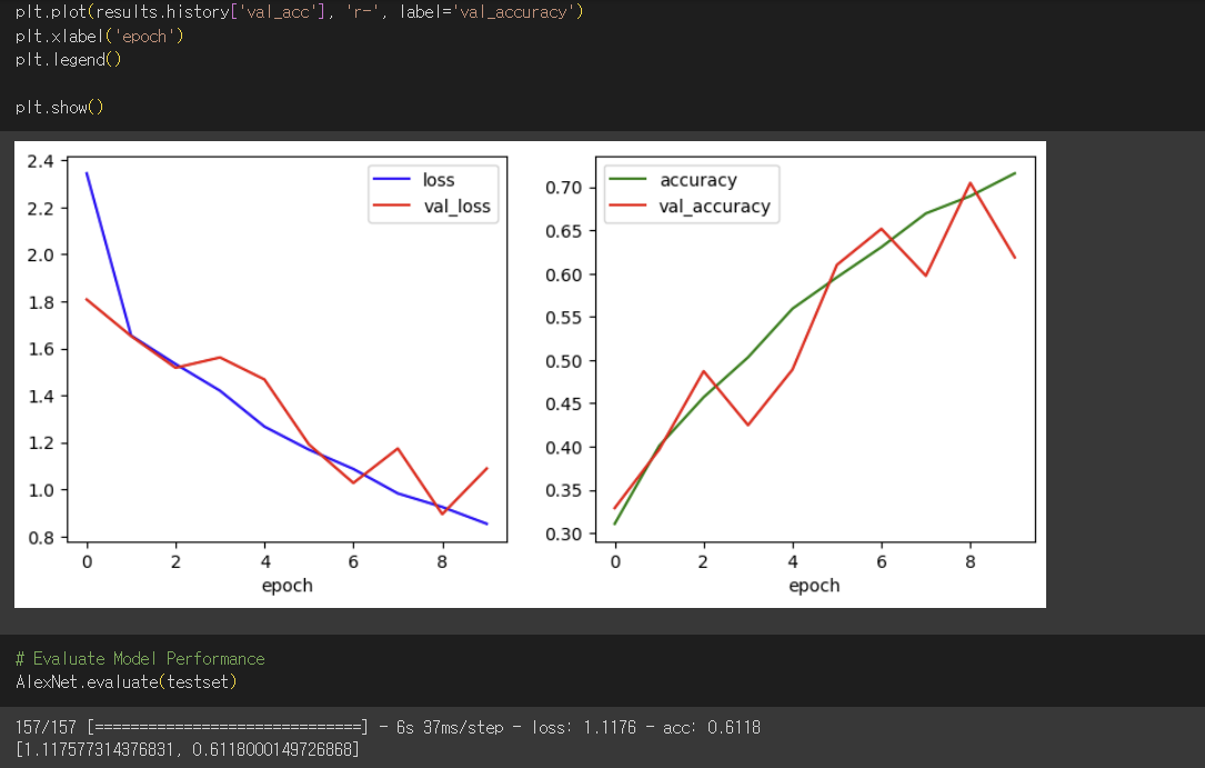
아래 내용은 learning rate를 변경했을 때
(다음과 같이 learning rate를 적절하게 증가시키면 정확도가 올라가고 loss가 낮아지는 것을 알 수 있는데
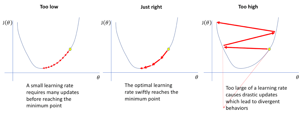
)
조절해보면서 대략적인 최대치를 찾아보기로 하였습니다.
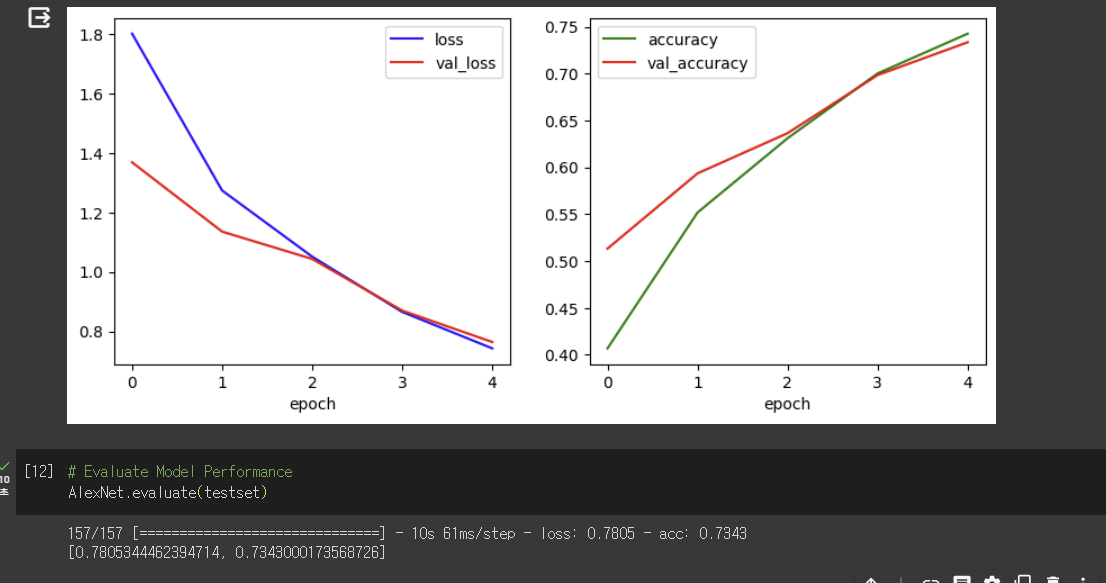
learning rate = 0.0001 일때는 다음과 같은 결과가 출력됩니다.
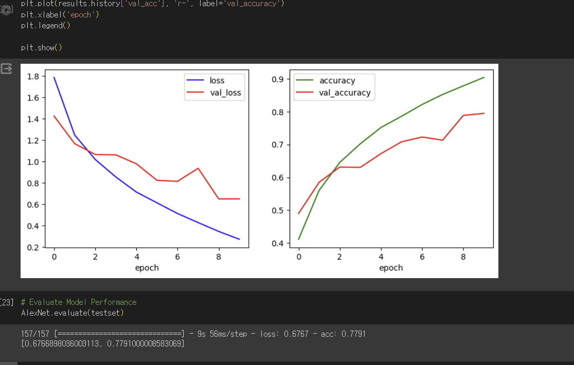
learning rate = 0.00005 일때는 다음과 같은 결과가 출력됩니다.
위의 결과로 미루어 볼 때 learning rate를 0.001보다는 0.0001로 하였을 때 보다 효과적인 것을 알 수 있고, 0.00005일때는 loss는 미세하게 떨어졌지만 acc는 떨어진 것으로보아 too low한 것이라고 생각되었습니다.
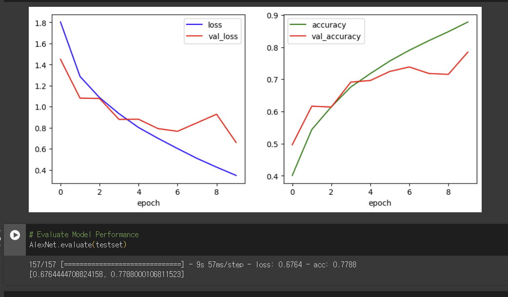
val_loss 와 loss 그리고 val_acc와 acc가 수렴도 안하고 차이가 꽤나 나는 것으로 보아 과적합이 일어나는 것 같아 epoch수를 5로 수정한 결과는 다음과 같습니다.
그리고 이후에 본래 8개의 layer로 구성되어있는 alexNet인데 마지막 layer 이전에 dense와 dropout을 진행하는 층을 추가한 결과 또한 비교하였습니다.
#Layer 8 (Dense)
tf.keras.layers.Dense(4096, activation='relu'), # Dense
tf.keras.layers.Dropout(0.5), # Dropout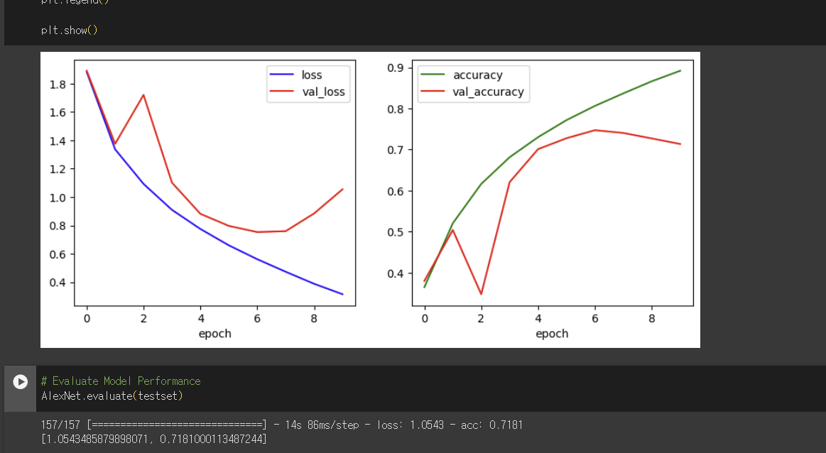
learning rate는 기본 0.0001인 것인데 다음과 같다. epoch수를 5로 줄였을떄는 다음과 같은 결과가 도출되었는데
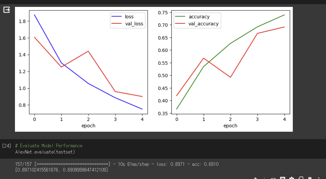
나와있는 결과들을 비교해 봤을 때 과적합이 일어나지 않으면서도 정확도와 loss가 가장 최적합일때의 결과는 learning rate가 0.0001이면서 epoch수가 5일때인 것으로 아주 조금 나아진 결과를 도출했습니다.
