구현할 것
- 공부시간과 성적간의 관계를 모델링한다.
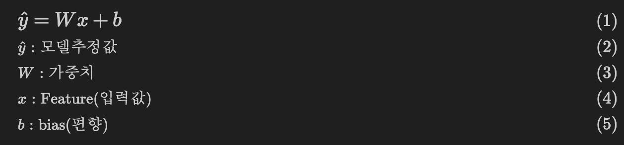
- 머신러닝 모델(모형)이란 수집한 데이터를 기반으로 입력값(Feature)와 출력값(Target)간의 관계를 하나의 공식으로 정의한 함수이다. 그 공식을 찾는 과정을 모델링이라고 한다.
- 이 예제에서는 공부한 시간으로 점수를 예측하는 모델을 정의한다.
- 입력값과 출력값 간의 관계를 정의할 수있는 다양한 함수(공식)이 있다. 여기에서는 딥러닝과 관계가 있는 Linear Regression 을 사용해본다.
데이터 확인
- 입력데이터: 공부시간
- 출력데이터: 성적
| 공부시간 | 점수 |
|---|---|
| 1 | 20 |
| 2 | 40 |
| 3 | 60 |
우리가 수집한 공부시간과 점수 데이터를 바탕으로 둘 간의 관계를 식으로 정의 할 수 있으면 내가 몇시간 공부하면 점수를 얼마 받을 수 있는지 예측할 수 있게 된다.
수집한 데이터를 기반으로 앞으로 예측할 수있는 모형을 만드는 것이 머신러닝 모델링이다.
학습(훈련) 데이터셋 만들기
- 모델을 학습시키기 위한 데이터셋을 구성한다.
- 입력데이터와 출력데이터을 각각 다른 행렬로 구성한다.
- 하나의 데이터 포인트의 입력/출력 값은 같은 index에 정의한다.
모델링
모델 정의
- Feature와 Target간의 관계를 수식으로 정의한다.
- 여기서는 공부시간(Feature)와 점수(Target)간의 관계를 정의하는데 선형회귀(Linear Regression) 모델 을 가설로 세우고 모델링을 한다.
- 많은 머신러닝 연구자들이 다양한 종류의 데이터간의 관계(패턴)를 예측할 수 있는 여러 알고리즘을 연구했다.
- 선형회귀 모델은 입력데이터와 출력데이터가 선형관계(linear)일때 좋은 성능을 나타낸다.
가설
- 아직은 이 식이 feature와 target의 관계를 잘 표현하는 함수인지 여부를 알 수없기 때문에 이 식을 가설(hypothesis) 라고 한다.
- 가설을 세우고 모델링을 한 뒤 검증을 해서 좋은 예측결과를 내면 그 가설을 최종 결과 모델로 결정한다. 예측결과가 좋지 않을 경우 새로운 가설로 모델링을 한다.
선형회귀 (Linear Regression)
- Feature들의 가중합을 이용해 Target을 추정한다.
- Feature에 곱해지는 가중치(weight)들은 각 Feature가 Target 얼마나 영향을 주는지 영향도가 된다.
- 음수일 경우는 target값을 줄이고 양수일 경우는 target값을 늘린다.
- 가중치가 0에 가까울 수록 target에 영향을 주지 않는 feature이고 0에서 멀수록 target에 많은 영향을 준다.
- 모델 학습과정에서 가장 적절한 Feature의 가중치를 찾아야 한다.
Train dataset 구성
- Train data는 feature(input)와 target(output) 각각 2개의 행렬로 구성한다.
- Feature의 행은 관측치(개별 데이터)를 열을 Feature(특성, 변수)를 표현한다. 이 문제에서는
공부시간1개의 변수를 가진다. - Target은 모델이 예측할 대상으로 행은 개별 관측치, 열은 각 항목에 대한 정답으로 구성한다. 이 문제에서 예측할 항목은
시험점수한개이다.
import torch
study_hours = [[1], [2], [3]]   # input (X)
scores = [[20],[40],[60]]        # output (y)
X_train = torch.tensor(study_hours, dtype=torch.float32)
y_train = torch.tensor(scores, dtype=torch.float32)
print(X_train.shape, y_train.size())
## (3:개수, 1:feature shape)
torch.Size([3, 1]) torch.Size([3, 1])
파라미터 (weight, bias) 정의
torch.manual_seed(0)
# W * X + b ==>
# Weight -> X feature 들에 곱해줄 가중치. X feature개수: 1 => weight: 1개
# bias -> 모든 feature들의 값이 0일 때 y의 값:   1개
## weight, bias가 경사하강법을 이용한 최적화 대상.  -> gradient를 구할 대상.
#       -> requires_grad=True
weight = torch.randn(1, 1, requires_grad=True)
# 1 - input shape(입력feature 개수)    X    1 - output shape(출력값의 개수)
bias = torch.randn(1, requires_grad=True)
print("------- 초기파라미터(weight, bias) ---------") # 랜덤값
print(f"Weight shape: {weight.shape}, Bias shape: {bias.shape}")
print("Weight:", weight)
print("Bias:", bias)
------- 초기파라미터(weight, bias) ---------
Weight shape: torch.Size([1, 1]), Bias shape: torch.Size([1])
Weight: tensor([[1.5410]], requires_grad=True)
Bias: tensor([-0.2934], requires_grad=True)model_pred = X_train @ weight + bias model_predtensor([[1.2476],
[2.7886],
[4.3296]], grad_fn=)y_traintensor([[20.],
[40.],
[60.]])
모델링
- 모델 정의 -> 선형회귀
- fitting -> 모델의 파라미터를 최적화. 경사하강법(gradient decent)
# 모델 정의
def linear_model(X) :
	return X @ weight + bias
# 오차 계산 함수 (Loss Function, Cost Function)
def loss_fn(pred, y):
	# 모델추정값과 정답을 받아서 오차 계산.
    ### 회귀 -> MSE (Mean Squared Error)
	return torch.mean((pred-y)**2)
# 모델로 추론 -> 오차 계산 pred = linear_model(X_train) loss = loss_fn(pred, y_train) print(pred) print(loss)tensor([[1.2476],
[2.7886],
[4.3296]], grad_fn=)
tensor(1611.8477, grad_fn=)# 손실 함수(loss)를 역전파(backpropagation)하여 # 모든 학습 가능한 매개변수(가중치와 편향)에 대한 기울기(gradient)를 계산 loss.backword() lr = 0.001 # 경사하강법 알고리즘 # weight를 업데이트 # weight.grad : 손실 함수에 대한 가중치의 기울기 # 기울기의 방향으로 가중치를 조정하여 손실을 줄인다. weight.data = weight.data - weight.grad * lr bias.data = bias.data - bias.grad * lrpred2 = linear_model(X_train) loss2 = loss_fn(pred2, y_train)losstensor(1611.8477, grad_fn=)
loss2tensor(1576.4189, grad_fn=)
학습
- 모델을 이용해 추정한다.
- pred = model(input)
- loss를 계산한다.
- loss = loss_fn(pred, target)
- 계산된 loss를 파라미터에 대해 미분하여 계산한 gradient 값을 각 파라미터에 저장한다.
- loss.backward()
- optimizer를 이용해 파라미터를 update한다.
- optimizer.step()
- 파라미터의 gradient(미분값)을 0으로 초기화한다.
- optimizer.zero_grad()
- 위의 단계를 반복한다.
torch.manual_seed(0)
# weight, bias
weight = torch.randn(1, 1, requires_grad=True)
bias = torch.randn(1, requires_grad=True)
# model def linear_model(X) : return X @ weight + bias # loss fn(손실함수) - MSE def loss_fn(pred, y) : return torch.mean((pred-y)**2)print(weight) print(bias)tensor([[1.5410]], requires_grad=True)
tensor([-0.2934], requires_grad=True)linear_model(X_train)tensor([[1.2476],
[2.7886],
[4.3296]], grad_fn=)epochs = 1000 # 반복횟수 lr = 0.01 for epoch in range(epochs) : # 1. 모델 추정 pred = linear_model(X_train) # 2. 오차 계산 loss = loss_fn(pred, y_train) # 3. parameter들의 gradient를 계산 loss.backward() # 4. parameter update ### weight update # weight.data: 현재값, weight.grad: gradient값 weight.data = weight.data - weight.grad * lr ### bias update bias.data = bias.data - bias.grad * lr # 5. weight, bias들의 gradient 값 초기화 weight.grad = None # weight.grad.zero_() bias.grad = None ##### 로그 출력(loss 값 출력) 100번 반복당 1회 출력 if epoch % 100 == 0 : print(f"[{epoch:03d}/{epochs}] loss - {loss}")[000/1000] loss - 1611.84765625
[100/1000] loss - 3.812145471572876
[200/1000] loss - 2.3556692600250244
[300/1000] loss - 1.4556654691696167
[400/1000] loss - 0.8995130062103271
[500/1000] loss - 0.555845320224762
[600/1000] loss - 0.34347668290138245
[700/1000] loss - 0.21224628388881683
[800/1000] loss - 0.13115528225898743
[900/1000] loss - 0.08104630559682846# 결과 확인 print("최종 loss: ", loss.item())최종 loss: 0.050322484225034714
print(weight) print(bias)tensor([[19.7401]], requires_grad=True)
tensor([0.5908], requires_grad=True)pred2 = linear_model(X_train) pred2tensor([[20.3309],
[40.0710],
[59.8111]], grad_fn=)y_traintensor([[20.],
[40.],
[60.]])
########################################
# 파이토치 optimizer를 이용해서 파라미터 업데이트
##    w.data = w.data - w.grad * lr   (이 작업을 처리하는 함수)
##    gradient 초기화.
torch.manual_seed(0)
# weight, bias
weight = torch.randn(1, 1, requires_grad=True)
bias = torch.randn(1, requires_grad=True)
# model
def linear_model(X) :
  	return X @ weight + bias
# loss_fn(손실함수) -MSE
def loss_fn(pred, y) :
  	return torch.mean((pred-y)**2)
# optimizer (instance) - 최적화대상 변수, learning rate
optim = torch.optim.SGD(
	[weight, bias], # 최적화 대상(requires_grad=True)
  	lr=0.01
)
a = torch.tensor(100)#### 학습 for epoch in range(epochs): # 1. 모델 추정 pred = linear_model(X_train) # 2. loss 계산 loss = loss_fn(pred, y_train) # 3. gradient 계산 - 역전파(backpropagation) loss.backward() # 4. 파라미터 최적화 -> optimizer.step() optim.step() # w.data = w.data - w.grade * lr, bias # 5. 파라미터 grad 값 초기화 optim.zero_grad() # log if epoch % 100 == 0 or epoch == 999: print(f"[{epoch:03d}/{1000}] - loss: {loss}")[000/1000] - loss: 1611.84765625
[100/1000] - loss: 3.812145471572876
[200/1000] - loss: 2.3556692600250244
[300/1000] - loss: 1.4556654691696167
[400/1000] - loss: 0.8995130062103271
[500/1000] - loss: 0.555845320224762
[600/1000] - loss: 0.34347668290138245
[700/1000] - loss: 0.21224628388881683
[800/1000] - loss: 0.13115528225898743
[900/1000] - loss: 0.08104630559682846
[999/1000] - loss: 0.050322484225034714
다중 입력, 다중 출력
- 다중입력: Feature가 여러개인 경우
- 다중출력: Output 결과가 여러개인 경우
다음 가상 데이터를 이용해 사과와 오렌지 수확량을 예측하는 선형회귀 모델을 정의한다.
참조
| 온도(F) | 강수량(mm) | 습도(%) | 사과생산량(ton) | 오렌지생산량 |
|---|---|---|---|---|
| 73 | 67 | 43 | 56 | 70 |
| 91 | 88 | 64 | 81 | 101 |
| 87 | 134 | 58 | 119 | 133 |
| 102 | 43 | 37 | 22 | 37 |
| 69 | 96 | 70 | 103 | 119 |
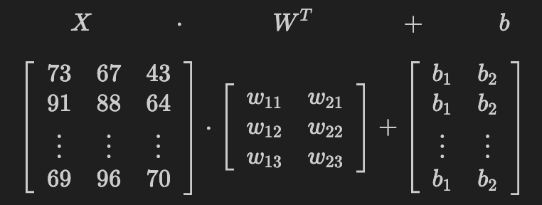
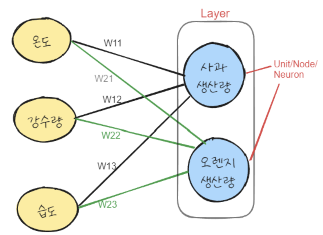
사과수확량  = w11 * 온도 + w12 * 강수량 + w13 * 습도 + b1
오렌지수확량 = w21 * 온도 + w22 * 강수량 + w23 *습도 + b2온도,강수량,습도값이 사과와, 오렌지 수확량에 어느정도 영향을 주는지 가중치를 찾는다.- 모델은 사과의 수확량, 오렌지의 수확량 두개의 예측결과를 출력해야 한다.
- 사과에 대해 예측하기 위한 weight 3개와 오렌지에 대해 예측하기 위한 weight 3개 이렇게 두 묶음, 총 6개의 weight를 정의하고 학습을 통해 가장 적당한 값을 찾는다.
개별 과일를 예측하기 위한 weight들 @ feature들의 계산 결과를 Node, Unit, Neuron 이라고 한다.- 두 과일에 대한 Unit들을 묶어서 Layer 라고 한다.
- 목적은 우리가 수집한 train 데이터셋을 이용해 정확한 예측을 위한 weight와 bias 들을 찾는 것이다.
Train Dataset
- Train data는 feature(input)와 target(output) 각각 2개의 행렬로 구성한다.
- Feature의 행은 관측치(개별 데이터)를 열을 Feature(특성, 변수)를 표현한다. 이 문제에서는
온도, 강수량, 습도세개의 변수를 가진다. - Target은 모델이 예측할 대상으로 행은 개별 관측치, 열은 각 항목에 대한 정답으로 구성한다. 이 문제에서 예측할 항목은
사과수확량, 오렌지 수확량2개의 값이다.
#  input: 생산환경 (temp, rainfall, humidity) : (5, 3)
environs = [
    [73, 67, 43],
    [91, 88, 64],
    [87, 134, 58],
    [102, 43, 37],
    [69, 96, 70]
]
# Targets: 생산량 - (apples, oranges) - (5, 2)
apple_orange_output = [
    [56, 70],
    [81, 101],
    [119, 133],
    [22, 37],
    [103, 119]
]
X = torch.tensor(environs, dtype=torch.float32) y = torch.tensor(apple_orange_output, dtype=torch.float32) X.shape, y.shape(torch.Size([5, 3]), torch.Size([5, 2]))
weight와 bias
- weight: 각 feature들이 생산량에 영향을 주었는지의 가중치로 feature에 곱해줄 값.
- 사과, 오렌지의 생산량을 구해야 하므로 가중치가 두개가 된다.
- weight의 shape:
(2, 3)
- bias는 모든 feature들이 0일때 생산량이 얼마일지를 나타내는 값으로 feature와 weight간의 가중합 결과에 더해줄 값이다.
- 사과, 오렌지의 생산량을 구하므로 bias가 두개가 된다.
- bias의 shape:
(2, )
# input: (N, 3)  weight: (3, 2)   3: feature들의 가중치개수, 2: 출력결과 개수(사과,오렌지)
### 행렬곱:  N x 2
weight = torch.randn(3, 2, requires_grad=True)
bias = torch.randn(2, requires_grad=True) # 사과, 오렌지 생산량에 각각 더할 bias
print(weight)
print(bias)
tensor([[-2.1788, 0.5684],
[-1.0845, -1.3986],
[ 0.4033, 0.8380]], requires_grad=True)
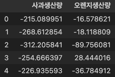
tensor([-0.7193, -0.4033], requires_grad=True)import pandas as pd result = X @ weight + bias print(result.shape) ### tensor.detach() : tensor객체를 gradient 계산 그래프에서 제거. (ndarray로 변경시 필요.) pd.DataFrame(result.detach().numpy(), columns=["사과생산량", "오렌지생산량"])torch.Size([5, 2])
Linear Regression model
모델은 weights w와 inputs x의 내적(dot product)한 값에 bias b를 더하는 함수.
weight = torch.randn(3, 2, requires_grad=True)
bias = torch.randn(2, requires_grad=True)
# model
def model(X):
    return X @ weight + bias
# loss 함수
def loss_fn(pred, y):
    # MSE
    return torch.mean((pred - y)**2)  # total loss -> 두 값의 오차를 합한다.
Gradients 계산
- loss에 대해 weight와 bias의 gradients (미분계수)를 계산한다.
- Pytorch의 자동미분을 이용한다. (graident를 구하려는 tensor는 requires_grad=True로 설정한다.)
모델 최적화(Optimize)
gradient decent 알고리즘을 이용해 loss를 줄여 모델의 추론 성능을 높인다. 이를 위해 좋은 성능을 낼 수 있도록 경사하강법(gradient decent) 을 이용해 weight와 bias를 update한다.
- 추론하기
- loss 계산하기
- weight와 bias에 대한 gradient계산하기
- 계산된 gradient에 비례한 값을 학습률을 곱해 작게 만든 뒤 wegith에서 빼서 조정한다.
- gradient를 0으로 초기화
epochs = 5000
lr = 0.00001  # 1e-5
for epoch in range(epochs):
    # 1. 추론
    pred = model(X)
    # 2. loss 계산
    loss = loss_fn(pred, y)
    # 3. gradient 계산
    loss.backward()
    # 4. update
    weight.data = weight.data - weight.grad * lr
    bias.data = bias.data - bias.grad * lr
    # 5. grad값 초기화.
    weight.grad.zero_()  # weight.grad = None
    bias.grad.zero_()
    if epoch % 100 == 0 or epoch == epochs-1:
        print(f"[{epoch:03d}/{epochs}] - loss: {loss}")
[000/5000] - loss: 36143.9296875
[100/5000] - loss: 180.45205688476562
[200/5000] - loss: 88.39179992675781
[300/5000] - loss: 56.189537048339844
[400/5000] - loss: 41.86906814575195
[500/5000] - loss: 33.46678924560547
[600/5000] - loss: 27.47199058532715
[700/5000] - loss: 22.7724666595459
[800/5000] - loss: 18.950511932373047
[900/5000] - loss: 15.801193237304688
[1000/5000] - loss: 13.194560050964355
[1100/5000] - loss: 11.033700942993164
[1200/5000] - loss: 9.24149227142334
[1300/5000] - loss: 7.754761695861816
[1400/5000] - loss: 6.521358489990234
[1500/5000] - loss: 5.498096942901611
[1600/5000] - loss: 4.649182319641113
[1700/5000] - loss: 3.944906711578369
[1800/5000] - loss: 3.3606231212615967
[1900/5000] - loss: 2.875887393951416
[2000/5000] - loss: 2.4737133979797363
[2100/5000] - loss: 2.1400771141052246
[2200/5000] - loss: 1.8632856607437134
[2300/5000] - loss: 1.6336517333984375
[2400/5000] - loss: 1.4431394338607788
...
[4700/5000] - loss: 0.5280918478965759
[4800/5000] - loss: 0.5259395837783813
[4900/5000] - loss: 0.5241520404815674
[4999/5000] - loss: 0.5226835608482361
Output is truncated. View as a scrollable element or open in a text editor. Adjust cell output settings...
pytorch built-in 모델을 사용해 Linear Regression 구현
import torch
import torch.nn as nn
inputs = torch.tensor(
    [[73, 67, 43],
     [91, 88, 64],
     [87, 134, 58],
     [102, 43, 37],
     [69, 96, 70]], dtype=torch.float32)
targets = torch.tensor(
    [[56, 70],
    [81, 101],
    [119, 133],
    [22, 37],
    [103, 119]], dtype=torch.float32)
nn.Linear
Pytorch는 nn.Linear 클래스를 통해 Linear Regression 모델을 제공한다.
nn.Linear에 입력 feature의 개수와 출력 값의 개수를 지정하면 random 값으로 초기화한 weight와 bias들을 생성해 모델을 구성한다.
Optimizer와 Loss 함수 정의
- torch.optim 모듈에 다양한 Optimizer 클래스가 구현되있다. 그 중에서 Adam를 사용한다.
- torch.nn 또는 torch.nn.functional 모듈에 다양한 Loss 함수가 제공된다. 이중 mse_loss() 를 사용한다.
## model: 선형회귀 -> nn.Linear()
model = nn.Linear(3, 2)  # 3: input feature 개수, 2: output 개수
# model.weight, model.bias
# model.parameters() # weight/bias를 generator로 반환.
## optimizer -> model의 parameter들을 넣어서 생성.
optim = torch.optim.SGD(
    model.parameters(), #최적화 대상 파라미터.
    lr=0.00001)
#### loss 함수 (nn.functional의 함수, nn 클래스)
loss_fn = nn.functional.mse_loss
Model Train
주어진 epoch 만큼 학습하는 fit 함수를 정의한다.
def fit(epochs, model, loss_fn, optim): """ epochs: 학습 반복 횟수 model: 학습시킬 대상 모델 loss_fn: loss function객체 optim: optimizer 객체 """ for epoch in range(epochs): pred = model(inputs) loss = loss_fn(pred, targets) # 추정값, 정답 loss.backward() optim.step() # 파라미터 업데이트 optim.zero_grad() # 파라미터 초기화. if epoch % 100 == 0 or epoch == epochs-1: print(f"[{epoch:03d}/{epochs}] - loss: {loss}")fit(5000, model, loss_fn, optim)[000/5000] - loss: 5417.5205078125
[100/5000] - loss: 140.97897338867188
[200/5000] - loss: 60.7963752746582
[300/5000] - loss: 34.740440368652344
[400/5000] - loss: 24.478763580322266
[500/5000] - loss: 19.151737213134766
[600/5000] - loss: 15.62641716003418
[700/5000] - loss: 12.95262622833252
[800/5000] - loss: 10.804781913757324
[900/5000] - loss: 9.042614936828613
[1000/5000] - loss: 7.586211204528809
[1100/5000] - loss: 6.379502773284912
[1200/5000] - loss: 5.3788251876831055
[1300/5000] - loss: 4.548752784729004
[1400/5000] - loss: 3.8601462841033936
[1500/5000] - loss: 3.2888665199279785
[1600/5000] - loss: 2.81492018699646
[1700/5000] - loss: 2.4217281341552734
[1800/5000] - loss: 2.0955140590667725
[1900/5000] - loss: 1.8248975276947021
[2000/5000] - loss: 1.600362777709961
[2100/5000] - loss: 1.4140926599502563
[2200/5000] - loss: 1.2595579624176025
[2300/5000] - loss: 1.131352186203003
[2400/5000] - loss: 1.0249972343444824
...
[4700/5000] - loss: 0.514125406742096
[4800/5000] - loss: 0.5129227042198181
[4900/5000] - loss: 0.5119251012802124
[4999/5000] - loss: 0.5111059546470642
Output is truncated. View as a scrollable element or open in a text editor. Adjust cell output settings...
