과적합, 일반화, 그리드서치

maro·2024년 5월 14일

머신러닝

과적합과 일반화

Generalization (일반화)
- 모델이 새로운 데이터셋(테스트 데이터)에 대하여 정확히 예측하면 이것을 일반화 되었다고 말한다.
  - 우리가 가진 데이터를 샘플(표본), 우리가 예측할 대상을 모집단 이라고 할 때 내가 가진 샘플 데이터셋이 아니라 모집단 전체에 대한 데이터의 일반적인 특성을 잘 학습한 모델의 상태를 일반화라고 한다.
- 모델이 훈련 데이터로 평가한 결과와 테스트 데이터로 평가한 결과의 차이가 거의 없고 좋은 평가결과를 보여준다.
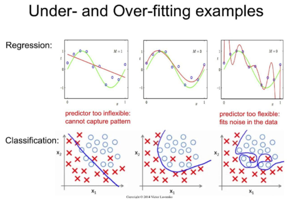
Overfitting (과대적합)
- 모델이 훈련 데이터에 대한 예측성능은 너무 좋지만 일반성이 떨어져 새로운 데이터(검증/테스트 데이터)에 대해선 성능이 좋지 않은 것을 Overfitting이라고 한다.
  - 훈련 데이터로 검증한 결과보다 검증데이터셋으로 검증한 결과가 현격하게 낮으면 Overfitting이 발생한 것이다.
- 이는 모델이 훈련 데이터 세트의 특징을 너무 맞춰서 학습 되었기 때문에 일반적으로 나타나지 않을 특징까지 학습되어 새로운 데이터(검증/테스트 셋)에 대한 예측 성능이 떨어지게 된다.
Underfitting (과소적합)
- 모델이 훈련 데이터과 테스트 데이터셋 모두에서 성능이 안좋은 것을 말한다.
- 모델이 너무 단순하여 훈련 데이터에 대해 충분히 학습하지 못해 데이터셋의 특성들을 다 찾아내지 못해서 발생한다.

Overfitting(과대적합)의 원인

학습 데이터 양에 비해 모델이 너무 복잡한 경우 발생.
- 데이터의 양을 늘린다.
  - 시간과 돈이 들기 때문에 현실적으로 어렵다.
- 모델을 좀더 단순하게 만든다.
  - 사용한 모델보다 좀더 단순한 모델을 사용한다.
  - 모든 모델은 모델의 복잡도를 변경할 수 있는 규제와 관련된 하이퍼파라미터를 제공하는데 이것을 조절한다.

Underfitting(과소적합)의 원인

데이터 양에 비해서 모델이 너무 단순한 경우 발생
- 좀더 복잡한 모델을 사용한다.
- 모델이 제공하는 규제 하이퍼파라미터를 조절한다.

모델 복잡도에 따른 성능 변화

출처: https://vitalflux.com/overfitting-underfitting-concepts-interview-questions/#google_vignette

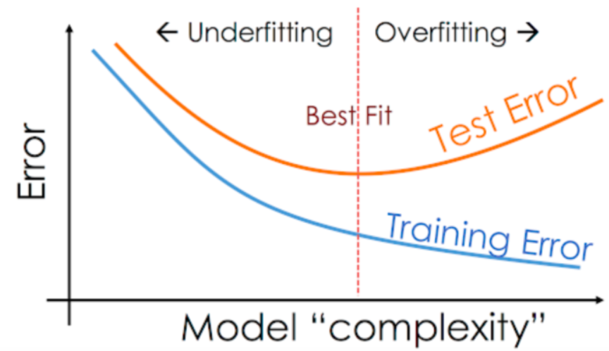
복잡한 모델, 단순한 모델

Overfitting 상태의 모델을 복잡한 모델, underfitting 상태의 모델을 단순한 모델 이라고 한다.

규제 하이퍼파라미터란?

모델의 복잡도를 규제하는 하이퍼파라미터로 Overfitting이나 Underfitting이 난 경우 이 값을 조정하여 모델이 일반화 되도록 도와준다.
이 규제 하이퍼파라미터들은 모든 머신러닝 모델마다 있다.

하이퍼파라미터란

하이퍼파라미터 (Hyper Parameter)

모델의 성능에 영향을 끼치는 파라미터 값으로 모델 생성시 사람이 직접 지정해 주는 값(파라미터)

하이퍼파라미터 튜닝(Hyper Parameter Tunning)

모델의 성능을 가장 높일 수 있는 하이퍼파라미터를 찾는 작업

파라미터(Parameter)

머신러닝에서 파라미터는 모델이 데이터 학습을 통해 직접 찾아야 하는 값을 말한다.

위스콘신 유방암 데이터셋 모델링

데이터 로딩 및 train/test set 분리

from sklearn.tree import DecisionTreeClassifier
from sklearn.metrics import accuracy_score
def tree_modeling(X, y, max_depth=None):
    """X, y 를 받아서 DecisionTree를 학습시키는 함수
    Parameter
        X: ndarray - features
        y: ndarray - label
        max_depth: int - DecisionTree의 규제하이퍼 파라미터.
    Return
        DecisionTreeClassifier: 학습한 D.Tree 모델 객체.
    """
    tree = DecisionTreeClassifier(max_depth=max_depth, random_state=0)
    tree.fit(X, y)
    return tree
def tree_accuracy(X, y, model, title):
    pred = model.predict(X)
    acc = accuracy_score(y, pred)
    print(f"{title}: {acc}")

tree5 = tree_modeling(X_train, y_train, 5)
print("max depth 5")
tree_accuracy(X_train, y_train, tree5, "Trainset")
tree_accuracy(X_test, y_test, tree5, "Testset")

max depth 5
Trainset: 1.0
Testset: 0.9020979020979021

from sklearn.tree import export_graphviz
from graphviz import Source
src = export_graphviz(
	tree5,										# 시각화할 DecisionTree 모델
    feature_names=data['feature_names']			# input feature들의 이름을 지정
    class_names=['악성', '양성'],	 			 # Label 클래스들(0, 1)의 클래스 이름(악성, 양성)을 지정.
    filled=True,								# 다수 클래스에 맞게 box를 색으로 채운다.
    rounded=True								# box모양(모서리 둥글게)
)
graph = Source(src)
graph

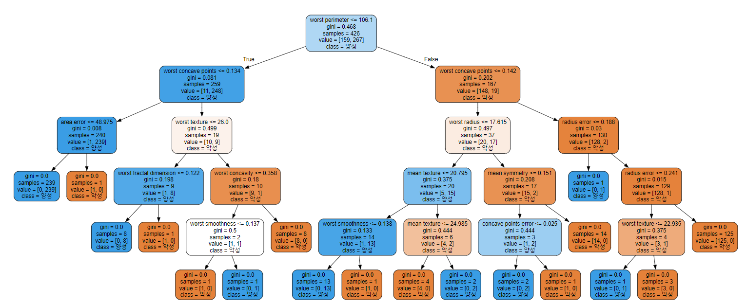
worst perimeter <= 106.1    # 현재 데이터셋(box안의 데이터들)을 분류하기 위한 질문
-----------------------------------------------------------
### 현재 데이터셋의 상태
gini = 0.468         # 지니계수: 불순도율을 계산한값.(각 클래스의 값들이 얼마나 섞여 있는지)
sample = 426       # 데이터 개수
value = [159, 267] # 클래스별 데이터 개수. 0: 159, 1: 267
class = 양성         # 다수 클래스의 클래스이름.

Decision Tree 복잡도 제어(규제 파라미터)

Decision Tree 모델을 복잡하게 하는 것은 노드가 너무 많이 만들어 지는 것이다.
- 노드가 많이 만들어 질수록 훈련데이터셋에 Overfitting 된다.
적절한 시점에 트리 생성을 중단해야 한다.
모델의 복잡도 관련 주요 하이퍼파라미터
- max_depth: 트리의 최대 깊이
- max_leaf_nodes : 리프노드 개수
- min_samples_leaf : leaf 노드가 되기위한 최소 샘플수

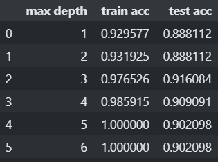
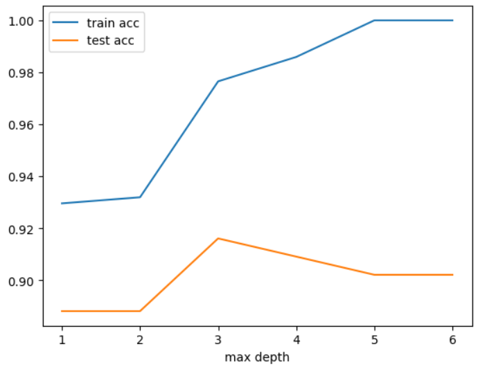
최적의 max_depth 찾기

# max_depth 는 작을 수록 규제를 강하게 한다.
### 규제를 강하게 한다. ==> 모델의 복잡도를 낮추는 방향으로 학습시키는 것.
max_depth_list = range(1, 7)
train_acc_list, test_acc_list = [], []
for max_depth in max_depth_list :
	model = DecisionTreeClassifier(max_depth=max_depth, random_state=0)
	model.fit(X_train, y_train)
    pred_train = model.predict(X_train)
    pred_test = model.predict(X_test)
    train_acc_list.append(accuracy_score(y_train, pred_train))
    test_acc_list.append(accuracy_score(y_test, pred_test))

import pandas as pd
result_df = pd.DataFrame({
    "max depth": max_depth_list,
    "train acc": train_acc_list,
    "test acc": test_acc_list
})
result_df

result_df.set_index('max depth').plot()

Grid Search 를 이용한 하이퍼파라미터 튜닝

모델의 성능을 가장 높게 하는 최적의 하이퍼파라미터를 찾는 방법.
하이퍼파라미터 후보들을 하나씩 입력해 모델의 성능이 가장 좋게 만드는 값을 찾는다.

종류

Grid Search 방식
- sklearn.model_selection.GridSearchCV
  - 시도해볼 하이퍼파라미터들을 지정하면 모든 조합에 대해 교차검증 후 제일 좋은 성능을 내는 하이퍼파라미터 조합을 찾아준다.
  - 적은 수의 조합의 경우는 괜찮지만 시도할 하이퍼파라미터와 값들이 많아지면 너무 많은 시간이 걸린다.
Random Search 방식
- sklearn.model_selection.RandomizedSearchCV
  - GridSeach와 동일한 방식으로 사용한다.
  - 모든 조합을 다 시도하지 않고 임의로 몇개의 조합만 테스트 한다.

GridSearchCV 매개변수및 결과조회

Initializer 매개변수
- estimator: 모델객체 지정
- params : 하이퍼파라미터 목록을 dictionary로 전달 '파라미터명':[파라미터값 list] 형식
- scoring: 평가 지표
  - 평가지표문자열: https://scikit-learn.org/stable/modules/model_evaluation.html#scoring-parameter
  - 생략시 분류는 accuracy, 회귀는 $R^2$ 를 기본 평가지표로 설정한다.
  - 여러개일 경우 List로 묶어서 지정
- refit: best parameter를 정할 때 사용할 평가지표
  - scoring에 여러개의 평가지표를 설정한 경우 refit을 반드시 설정해야 한다.
- cv: 교차검증시 fold 개수.
- n_jobs: 사용할 CPU 코어 개수 (None:1(기본값), -1: 모든 코어 다 사용)
메소드
- fit(X, y): 학습
- predict(X): 분류-추론한 class. 회귀-추론한 값
  - 제일 좋은 성능을 낸 모델로 predict()
- predict_proba(X): 분류문제에서 class별 확률을 반환
  - 제일 좋은 성능을 낸 모델로 predict_proba() 호출
결과 조회 속성
- fit() 후에 호출 할 수 있다.
- cvresults: 파라미터 조합별 평가 결과를 Dictionary로 반환한다.
- bestparams: 가장 좋은 성능을 낸 parameter 조합을 반환한다.
- bestestimator: 가장 좋은 성능을 낸 모델을 반환한다.
- bestscore: 가장 좋은 점수 반환한다.

데이터셋 로드 및 train/test set 나누기

from sklearn.datasets import load_breast_cancer
from sklearn.model_selection import train_test_split
data = load_breast_cancer()
X, y = data.data, data.target
X_train, X_test, y_train, y_test = train_test_split(X, y, stratify=y, random_state=0)
GridSearchCV 생성
from sklearn.model_selection import GridSearchCV
# 최적의 하이퍼파라미터를 찾을 대상 모델
model = DecisionTreeClassifier(random_state=0)
# 파라미터 후보: dictionary - key: 하이퍼파라미터이름, value: 후보리스트
params = {
	"max_depth":range(1, 6),
    "max_leaf_nodes":range(3, 11)
}
# GridSearchCV 생성
gs = GridSearchCV(
	model, 					# 대상 모델
    params,					# 하이퍼파라미터 후보
    scoring="accuracy",		# 평가지표(default: 분류-accuracy, 회귀: r2), 평가지표가 여러개일 경우 리스트에 묶어서 전달.		
    cv=4,					# Cross Validation의 folder 개수
    n_jobs=-1				# 학습할 때 병렬처리. 프로세스(cpu) 개수 지정. -1 : 모든 프로세스 다 사용.
)
학습
gs.fit(X_train, y_train)
결과확인
#### 가장 성능 좋은 hyper parameter 조합
gs.best_params_
{'max_depth': 2, 'max_leaf_nodes': 4}
#### 가장 좋은 성능의 하이퍼파라미터를 사용했을때 성능점수(정확도)
gs.best_score_
0.9248809733733028
### 모든 조합에 대한 평가 결과
import pandas as pd
result = pd.DataFrame(gs.cv_results_)
result.sort_values('rank_test_score')
mean_fit_time std_fit_time mean_score_time std_score_time param_max_depth param_max_leaf_nodes params split0_test_score split1_test_score split2_test_score split3_test_score mean_test_score std_test_score rank_test_score
11 0.003691 0.000864 0.000329 0.000569 2 6 {'max_depth': 2, 'max_leaf_nodes': 6} 0.897196 0.953271 0.905660 0.943396 0.924881 0.023899 1
15 0.000000 0.000000 0.000000 0.000000 2 10 {'max_depth': 2, 'max_leaf_nodes': 10} 0.897196 0.953271 0.905660 0.943396 0.924881 0.023899 1
14 0.004650 0.002685 0.000000 0.000000 2 9 {'max_depth': 2, 'max_leaf_nodes': 9} 0.897196 0.953271 0.905660 0.943396 0.924881 0.023899 1
13 0.004650 0.002685 0.001502 0.002602 2 8 {'max_depth': 2, 'max_leaf_nodes': 8} 0.897196 0.953271 0.905660 0.943396 0.924881 0.023899 1
12 0.000329 0.000569 0.000000 0.000000 2 7 {'max_depth': 2, 'max_leaf_nodes': 7} 0.897196 0.953271 0.905660 0.943396 0.924881 0.023899 1
9 0.006369 0.000178 0.001256 0.000183 2 4 {'max_depth': 2, 'max_leaf_nodes': 4} 0.897196 0.953271 0.905660 0.943396 0.924881 0.023899 1
10 0.004647 0.001672 0.001137 0.000283 2 5 {'max_depth': 2, 'max_leaf_nodes': 5} 0.897196 0.953271 0.905660 0.943396 0.924881 0.023899 1
26 0.003030 0.000706 0.000750 0.000433 4 5 {'max_depth': 4, 'max_leaf_nodes': 5} 0.906542 0.925234 0.915094 0.943396 0.922567 0.013726 8
34 0.008558 0.007853 0.000128 0.000221 5 5 {'max_depth': 5, 'max_leaf_nodes': 5} 0.906542 0.925234 0.915094 0.943396 0.922567 0.013726 8
17 0.006543 0.004452 0.000252 0.000436 3 4 {'max_depth': 3, 'max_leaf_nodes': 4} 0.897196 0.953271 0.905660 0.933962 0.922522 0.022372 10
33 0.004745 0.006844 0.004064 0.006531 5 4 {'max_depth': 5, 'max_leaf_nodes': 4} 0.897196 0.953271 0.905660 0.933962 0.922522 0.022372 10
25 0.003296 0.000852 0.000250 0.000433 4 4 {'max_depth': 4, 'max_leaf_nodes': 4} 0.897196 0.953271 0.905660 0.933962 0.922522 0.022372 10
39 0.000000 0.000000 0.000000 0.000000 5 10 {'max_depth': 5, 'max_leaf_nodes': 10} 0.906542 0.915888 0.896226 0.962264 0.920230 0.025245 13
18 0.002637 0.000482 0.000366 0.000417 3 5 {'max_depth': 3, 'max_leaf_nodes': 5} 0.906542 0.925234 0.915094 0.933962 0.920208 0.010336 14
28 0.002017 0.002145 0.000267 0.000462 4 7 {'max_depth': 4, 'max_leaf_nodes': 7} 0.925234 0.906542 0.896226 0.952830 0.920208 0.021514 15
30 0.000517 0.000895 0.000000 0.000000 4 9 {'max_depth': 4, 'max_leaf_nodes': 9} 0.915888 0.915888 0.896226 0.952830 0.920208 0.020473 15
38 0.000000 0.000000 0.000000 0.000000 5 9 {'max_depth': 5, 'max_leaf_nodes': 9} 0.915888 0.915888 0.896226 0.952830 0.920208 0.020473 15
36 0.005097 0.007447 0.000000 0.000000 5 7 {'max_depth': 5, 'max_leaf_nodes': 7} 0.925234 0.906542 0.896226 0.952830 0.920208 0.021514 15
32 0.000000 0.000000 0.000000 0.000000 5 3 {'max_depth': 5, 'max_leaf_nodes': 3} 0.897196 0.953271 0.896226 0.933962 0.920164 0.024428 19
16 0.000000 0.000000 0.002468 0.004274 3 3 {'max_depth': 3, 'max_leaf_nodes': 3} 0.897196 0.953271 0.896226 0.933962 0.920164 0.024428 19
8 0.011419 0.003498 0.001096 0.000153 2 3 {'max_depth': 2, 'max_leaf_nodes': 3} 0.897196 0.953271 0.896226 0.933962 0.920164 0.024428 19
24 0.002782 0.000413 0.000000 0.000000 4 3 {'max_depth': 4, 'max_leaf_nodes': 3} 0.897196 0.953271 0.896226 0.933962 0.920164 0.024428 19
35 0.008937 0.008937 0.000000 0.000000 5 6 {'max_depth': 5, 'max_leaf_nodes': 6} 0.906542 0.906542 0.915094 0.943396 0.917894 0.015132 23
27 0.002767 0.001914 0.000267 0.000462 4 6 {'max_depth': 4, 'max_leaf_nodes': 6} 0.906542 0.906542 0.915094 0.943396 0.917894 0.015132 23
19 0.000328 0.000359 0.000000 0.000000 3 6 {'max_depth': 3, 'max_leaf_nodes': 6} 0.906542 0.906542 0.915094 0.943396 0.917894 0.015132 23
29 0.001393 0.001483 0.000141 0.000243 4 8 {'max_depth': 4, 'max_leaf_nodes': 8} 0.915888 0.915888 0.886792 0.952830 0.917850 0.023430 26
37 0.000128 0.000221 0.000000 0.000000 5 8 {'max_depth': 5, 'max_leaf_nodes': 8} 0.915888 0.915888 0.886792 0.952830 0.917850 0.023430 26
22 0.005032 0.002108 0.000250 0.000432 3 9 {'max_depth': 3, 'max_leaf_nodes': 9} 0.897196 0.906542 0.915094 0.943396 0.915557 0.017274 28
21 0.002997 0.003083 0.001755 0.001904 3 8 {'max_depth': 3, 'max_leaf_nodes': 8} 0.897196 0.906542 0.915094 0.943396 0.915557 0.017274 28
23 0.002883 0.000334 0.000201 0.000349 3 10 {'max_depth': 3, 'max_leaf_nodes': 10} 0.897196 0.906542 0.915094 0.943396 0.915557 0.017274 28
20 0.003019 0.002845 0.000000 0.000000 3 7 {'max_depth': 3, 'max_leaf_nodes': 7} 0.897196 0.906542 0.905660 0.943396 0.913199 0.017812 31
31 0.000000 0.000000 0.003840 0.006650 4 10 {'max_depth': 4, 'max_leaf_nodes': 10} 0.887850 0.915888 0.896226 0.952830 0.913199 0.025042 31
7 0.004509 0.004509 0.005872 0.003146 1 10 {'max_depth': 1, 'max_leaf_nodes': 10} 0.841121 0.906542 0.905660 0.896226 0.887388 0.027016 33
6 0.001385 0.001675 0.000567 0.000982 1 9 {'max_depth': 1, 'max_leaf_nodes': 9} 0.841121 0.906542 0.905660 0.896226 0.887388 0.027016 33
5 0.004332 0.000287 0.001844 0.001139 1 8 {'max_depth': 1, 'max_leaf_nodes': 8} 0.841121 0.906542 0.905660 0.896226 0.887388 0.027016 33
4 0.008138 0.002961 0.005684 0.002498 1 7 {'max_depth': 1, 'max_leaf_nodes': 7} 0.841121 0.906542 0.905660 0.896226 0.887388 0.027016 33
3 0.002656 0.002671 0.000224 0.000388 1 6 {'max_depth': 1, 'max_leaf_nodes': 6} 0.841121 0.906542 0.905660 0.896226 0.887388 0.027016 33
2 0.006734 0.001539 0.002107 0.000759 1 5 {'max_depth': 1, 'max_leaf_nodes': 5} 0.841121 0.906542 0.905660 0.896226 0.887388 0.027016 33
1 0.003572 0.001669 0.001643 0.001877 1 4 {'max_depth': 1, 'max_leaf_nodes': 4} 0.841121 0.906542 0.905660 0.896226 0.887388 0.027016 33
0 0.001430 0.002476 0.004128 0.006642 1 3 {'max_depth': 1, 'max_leaf_nodes': 3} 0.841121 0.906542 0.905660 0.896226 0.887388 0.027016 33
##### 가장 좋은 하이퍼파라미터로 학습한 모델을 조회
best_model = gs.best_estimator_
best_model
best model을 이용해 Test set 최종평가
pred = best_model.predict(X_test)
accuracy_score(y_test, pred)
0.8881118881118881
pred2 = gs.predict(X_test)  # best_estimator_ 모델을 이용해 추정.
accuracy_score(y_test, pred2)
0.8881118881118881

여러 성능지표를 확인

여러 성능지표는 확인할 수 있지만 최적의 파라미터를 찾기 위해서는 하나의 지표만 사용한다.
- scoring에 리스트로 평가지표들 묶어서 설정
- refit에 최적의 파라미터 찾기 위한 평가지표 설정

GridSearchCV 생성

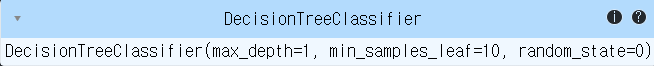
model = DecisionTreeClassifier(random_state=0)
params = {
    "max_depth": range(1, 5), 
    "min_samples_leaf": [10, 20, 30, 40, 50]
}
gs2 = GridSearchCV(
    model, params, 
    scoring= ["accuracy", "recall", "precision"], # 평가지표가 여러개이면 리스트로 묶어서 전달.
    refit="recall", # 순위의 기준이 되는 평가 지표를 지정. 
# 이 지표 성능이 가장 좋은 하이퍼파라미터로 모델을 재학습해서 best_estimator_에 할당한다.
    cv=4, 
    n_jobs=-1
)
gs2.fit(X_train, y_train)

결과확인

gs2.best_params_

{'max_depth': 1, 'min_samples_leaf': 10}

gs2.best_score_

0.9252035278154681

gs2.best_estimator_

업로드중..

RandomizedSearchCV

Initializer 매개변수
- estimator: 모델객체 지정
- param_distributions: 하이퍼파라미터 목록을 dictionary로 전달 '파라미터명':[파라미터값 list] 형식
- n_iter: 전체 조합중 몇개의 조합을 테스트 할지 개수 설정
- scoring: 평가 지표
- refit: best parameter를 정할 때 사용할 평가지표. Scoring에 여러개의 평가지표를 설정한 경우 설정.
- cv: 교차검증시 fold 개수.
- n_jobs: 사용할 CPU 코어 개수 (None:1(기본값), -1: 모든 코어 다 사용)
메소드
- fit(X, y): 학습
- predict(X): 분류-추론한 class. 회귀-추론한 값
  - 제일 좋은 성능을 낸 모델로 predict()
- predict_proba(X): 분류문제에서 class별 확률을 반환
  - 제일 좋은 성능을 낸 모델로 predict_proba() 호출
결과 조회 속성
- fit() 후에 호출 할 수 있다.
- cvresults: 파라미터 조합별 평가 결과를 Dictionary로 반환한다.
- bestparams: 가장 좋은 성능을 낸 parameter 조합을 반환한다.
- bestestimator: 가장 좋은 성능을 낸 모델을 반환한다.
- bestscore: 가장 좋은 점수 반환한다.

from sklearn.datasets import load_breast_cancer
from sklearn.model_selection import train_test_split
data = load_breast_cancer()
X, y = data.data, data.target
X_train, X_test, y_train, y_test = train_test_split(X, y, stratify=y, random_state=0)

from sklearn.model_selection import RandomizedSearchCV
import numpy as np
model = DecisionTreeClassifier(random_state=0)
params = {
    "max_depth": range(1, 6), 
    "max_leaf_nodes": range(3, 30),
    "max_features": np.arange(0.1, 1.1, 0.1), # 학습할 때 사용할 feature(컬럼)의 개수(비율)
}
rs = RandomizedSearchCV(
    model, # 하이퍼파라미터를 찾을 모델
    params, # 하이퍼파라미터 후보들 (dict: key-하이퍼파라미터이름, value-후보리스트)
    n_iter=60, # 테스트할 하이퍼파라미터 조합 개수 (random하게 조합을 선택.)
    scoring="accuracy", # 평가지표
    cv=4, # cross validation fold 개수
    n_jobs=-1
)
rs.fit(X_train, y_train)

결과확인

print("best parameter:", rs.best_params_)
print("best score:", rs.best_score_)

best parameter: {'max_leaf_nodes': 16, 'max_features': 0.4, 'max_depth': 5}
best score: 0.9530285663904072

best model을 이용해 Test set 최종평가

best_model = rs.best_estimator_
accuracy_score(y_test, best_model.predict(X_test))

0.9440559440559441

accuracy_score(y_test, rs.predict(X_test))

maro

공부 & 프로젝트 & 개발 블로그

이전 포스트

데이터 전처리

다음 포스트

과적합, 일반화, 그리드서치

과적합과 일반화

Overfitting(과대적합)의 원인

Underfitting(과소적합)의 원인

모델 복잡도에 따른 성능 변화

규제 하이퍼파라미터란?

하이퍼파라미터란

위스콘신 유방암 데이터셋 모델링

데이터 로딩 및 train/test set 분리

Decision Tree 복잡도 제어(규제 파라미터)

최적의 max_depth 찾기

Grid Search 를 이용한 하이퍼파라미터 튜닝

종류

GridSearchCV 매개변수및 결과조회

데이터셋 로드 및 train/test set 나누기

GridSearchCV 생성

학습

결과확인

best model을 이용해 Test set 최종평가

여러 성능지표를 확인

GridSearchCV 생성

결과확인

RandomizedSearchCV

결과확인

best model을 이용해 Test set 최종평가

데이터 전처리

파이프라인

0개의 댓글