파이프라인 (Pipeline)

• 개요
  • 여러 단계의 머신러닝 프로세스 (전처리의 각 단계, 모델생성, 학습) 처리 과정을 설정하여 한번에 처리되도록 한다.
• 파이프라인은 여러개의 변환기와 마지막에 변환기 또는 추정기를 넣을 수 있다. (추정기-Estimator는 마지막에만 올 수 있다.)
• 전처리 작업 파이프라인
  • 변환기들로만 구성
• 전체 프로세스 파이프 라인
  • 마지막에 추정기를 넣는다

Pipeline 생성

• (이름, 변환기) 를 리스트로 묶어서 전달한다.
• 마지막에는 추정기가 올 수있다.

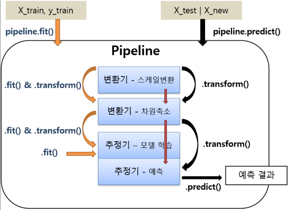
Pipeline 을 이용한 학습

• pipeline.fit()
  • 각 순서대로 각 변환기의 fit_transform()이 실행되고 결과가 다음 단계로 전달된다. 마지막 단계에서는 fit()만 호출한다.
  • 마지막이 추정기일때 사용
• pipeline.fit_transform()
  • fit()과 동일하나 마지막 단계에서도 fit_transform()이 실행된다.
  • 전처리 작업 파이프라인(모든 단계가 변환기)일 때 사용
• 마지막이 추정기(모델) 일 경우
  • predict(X), predict_proba(X)
  • 추정기를 이용해서 X에 대한 결과를 추론
  • 모델 앞에 있는 변환기들을 이용해서 transform() 그 처리결과를 다음 단계로 전달

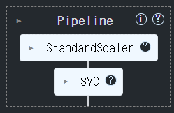
from sklearn.datasets import load_breast_cancer
from sklearn.model_selection import train_test_split
data = load_breast_cancer()
X, y = data.data, data.target
X_train, X_test, y_train, y_test = train_test_split(X, y, stratify=y, random_state=0)

Pipeline 생성

from sklearn.pipeline import Pipeline
from sklearn.preprocessing import StandardScaler # 전처리기(변환기)
from sklearn.svm import SVC # 모델(추정기)
# pipeline 생성
## 머신러닝 프로세스를 담당하는 객체들(변환기, 추정기-마지막프로세스) 를 순서대로 묶어서 생성.
### [(이름, 객체), (이름, 객체), ... ]  ==> OrderedDict (순서가 있는 딕셔너리)
steps = [
	("scaler", StandardScaler()), ### 1번째 프로세스 담당.
    ("svm", SVC(random_state=0)) ### 2번째 프로세스 담당.
]
pipeline = Pipeline(steps, verbose=True) # verbose : 학습 상황을 출력(log 기록 출력)
### pipeline 구성 step들 조회
p_steps = pipeline.steps
print(type(p_steps))
p_steps

<class 'list'>
[('scaler', StandardScaler()), ('svm', SVC(random_state=0))]

학습

pipeline.fit(X_train, y_train)
###  1단계) x = scaler.fit_transform(X_train)  2단계) svm.fit(x: 1단계에서변환된값, y_train)

[Pipeline] ............ (step 1 of 2) Processing scaler, total= 0.0s
[Pipeline] ............... (step 2 of 2) Processing svm, total= 0.0s

추론 및 평가

### 추론 - trainset 검증
pred_train = pipeline.predict(X_train)
### 1단계) x =  scaler.transform(X_train) , 2단계)  pred = svm.predict(x : 1단계 처리값) 
######### pred를 리턴.
#### testset 검증
pred_test = pipeline.predict(X_test)

from sklearn.metrics import accuracy_score
print(accuracy_score(y_train, pred_train))
print(accuracy_score(y_test, pred_test))

0.9929577464788732
0.958041958041958

##### 모델을 파일에 저장(pickle) => Pipeline을 저장.
import pickle, os
os.makedirs("saved_models", exist_ok=True)
with open('saved_models/breast_cancer_pipeline.pkl', "wb") as fo:
    pickle.dump(pipeline, fo)

with open('saved_models/breast_cancer_pipeline.pkl', 'rb') as fi:
    saved_pipeline = pickle.load(fi)
accuracy_score(y_test, saved_pipeline.predict(X_test))

0.958041958041958

GridSearch에서 Pipeline 사용

• 하이퍼파라미터 지정시 파이프라인 프로세스이름__하이퍼파라미터 형식으로 지정한다.

1. Pipeline 생성
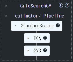
2. GridSearchCV의 estimator에 pipeline 등록

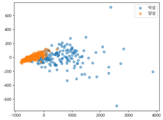
# PCA : 전처리-비지도학습 알고리즘중 하나.
# 차원축소 ==> 기존 feature들의 정보를 최대한 유지하면서 feature 개수를 줄여준다.
## 컬럼 수 줄이기: 
##### feature selection(feature를 선택-선택된 feature의 원래값을 유지),
##### feature extraction(계산을 통해서 줄이기.-원래 feature의 값이 변경.)
from sklearn.decomposition import PCA # feature extraction
pca = PCA(n_components=2) # feature를 몇개로 줄일지
pca.fit(X_train)
t1 = pca.transform(X_train)
t2 = pca.transform(X_test)
X_train.shape, t1.shape, X_test.shape, t2.shape

((426, 30), (426, 2), (143, 30), (143, 2))

import matplotlib.pyplot as plt
plt.rcParams['font.family'] = "malgun gothic"
plt.rcParams['axes.unicode_minus'] = False
zero_index = np.where(y_train==0)[0]    # 레이블 값에 따른 index
one_index = np.where(y_train==1)[0]      
# zero_index: 0으로 표시된 샘플의 인덱스 포함(악성)
# 악성(음수) 클래스에 해당하는 점의 x 및 y 좌표
# t1[zero_index, 0]"악성"으로 레이블이 지정된 샘플의 첫 번째 주성분 값
# t1[zero_index, 1]동일한 표본에 대한 두 번째 주성분 값
plt.scatter(t1[zero_index, 0], t1[zero_index, 1], label="악성", alpha=0.5) 
plt.scatter(t1[one_index, 0], t1[one_index, 1], label="양성", alpha=0.5)
plt.legend()
plt.show()

Pipeline 생성

## 변환기 - 1) StandardScaler -> 2) PCA (n_components: 2 ~ 30)
##  추정기 - 3) SVM (c, gamma)
stpes = [
	("scaler", StandardScaler()),
    ("pca", PCA()),
    ("svm", SVC(random_state=0))
]
pipeline = Pipeline(steps, verbose=True)

GridSearchCV 생성

params = {
	"pca__n_components": range(2, 31),  #PCA
    "svm__C":[0.01, 0.1, 0.5, 1],               #SVC
    "svm__gamma":[0.01, 0.1, 0.5, 1]        #SVC
}
gs = GridSearchCV(
    pipeline, # 모델에 pipeline을 지정.
    params, 
    scoring="accuracy", 
    cv=4, 
    n_jobs=-1
)

학습

gs.fit(X_train, y_train)

[Pipeline] ............ (step 1 of 3) Processing scaler, total= 0.0s
[Pipeline] ............... (step 2 of 3) Processing pca, total= 0.0s
[Pipeline] ............... (step 3 of 3) Processing svm, total= 0.0s

결과확인

gs.best_params_

{'pcan_components': 5, 'svmC': 1, 'svm__gamma': 0.1}

gs.best_score_

0.9765914300828777

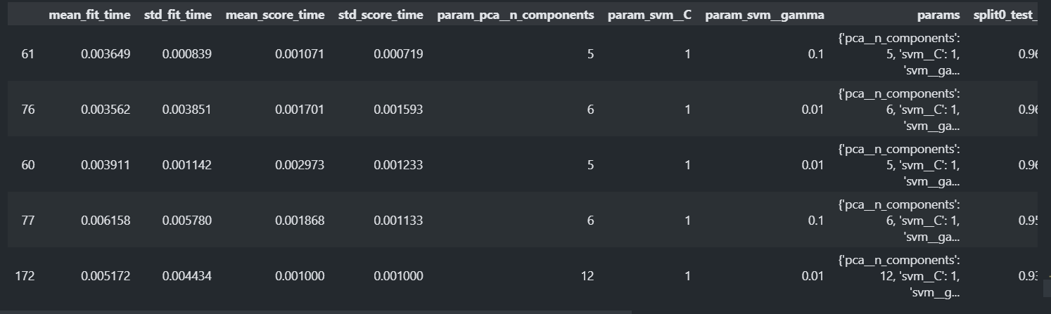
result_df = pd.DataFrame(gs.cv_results_)
result_df.sort_values("rank_test_score").head()

best_model = gs.best_estimator_
type(best_model)

sklearn.pipeline.Pipeline

accuracy_score(y_test, best_model.predict(X_test))

0.9440559440559441

make_pipeline() 함수를 이용한 파이프라인 생성을 편리하게 하기

• make_pipeline(변환기객체, 변환기객체, ....., 추정기객체): Pipeline
• 프로세스의 이름을 프로세스클래스이름(소문자로변환)으로 해서 Pipeline을 생성.

from sklearn.pipeline import make_pipeline
pipeline = make_pipeline(
	StandardScaler(),
    PCA(n_components=5),
    SVC()
)
print(pipeline.steps)

[('standardscaler', StandardScaler()), ('pca', PCA(n_components=5)), ('svc', SVC())]

ColumnTransformer

• 데이터셋의 컬럼들 마다 다른 전처리를 해야 하는 경우 사용한다.
  • 연속형 feature들은 feature scaling을 범주형은 one hot encoding이나 label encoding을 해야한다. 또한 결측치 처리하는 방법도 다르다. 그런데 대부분의 데이터셋은 그 두가지 타입의 feature들을 모두 가지고 있다. 그래서 전처리시 나눠서 처리후 합치는 번거로운 작업이 필요하다.
  • 위의 예처럼 하나의 데이터셋을 구성하는 feature들(컬럼들)에 대해 서로 다른 전처리 방법이 필요할 때 개별적으로 나눠서 처리하는 것은 다음과 같은 이유에서 좋지 않다.
    1. 번거롭다.
    2. 전처리 방식을 저장할 수 없다.
    3. Pipeline을 구성하여 한번에 처리할 수 없다.
  • ColumnTransformer를 사용하면 feature별로 어떤 전처리를 할지 정의할 수 있다.

sklearn.compose.ColumnTransformer 이용

• 매개변수
  • transformer: list of tuple - (name, transformer, columns)로 구성된 tuple들을 리스트로 묶어 전달한다.
  • remainder='drop' : 지정하지 않은 컬럼을 어떻게 처리할지 여부
    • "drop"(기본값): 제거한다.
    • "passthrough": 남겨둔다.

sklearn.compose.make_column_transformer 이용

• ColumnTransformer를 쉽게 생성할 수 있도록 도와주는 utility 함수
• 매개변수
  • transformer: 가변인자. (transformer, columns 리스트)로 구성된 tuple을 전달한다.
  • remainder='drop' : 컬럼 리스트에 지정되지 않은 컬럼을 어떻게 처리할지 여부
    • "drop"(기본값): 제거한다.
    • "passthrough": 남겨둔다.
• 반환값: ColumnTransformer

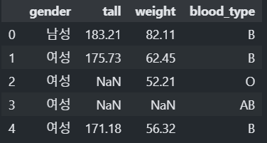
# dummy dataset
import pandas as pd
import numpy as np
df = pd.DataFrame({
    "gender":['남성', '여성', '여성', '여성', '여성', '여성', '남성', np.nan],
    "tall":[183.21, 175.73, np.nan, np.nan, 171.18, 181.11, 168.83, 193.99],
    "weight":[82.11, 62.45, 52.21, np.nan, 56.32, 48.93, 63.64, 102.38],
    "blood_type":["B", "B", "O", "AB", "B", np.nan, "B", "A"],
})
df.head()

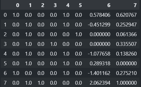
from sklearn.compose import ColumnTransformer
from sklearn.impute import SimpleImputer # 결측치값 대체.
from sklearn.preprocessing import OneHotEncoder, StandardScaler, MinMaxScaler
# 전처리별로 생성
### 결측치 처리. - 컬럼별로 다르게 처리
### [("전처리기 이름",  전처리기, 리스트[컬럼명])]
na_transformer = ColumnTransformer([
    ("category_imputer", SimpleImputer(strategy="most_frequent"), ["gender", "blood_type"]),
    ("number_imputer", SimpleImputer(strategy="mean"), ["tall", "weight"])
])
### 순서대로 변환 하고 단순히 합친다.
##### 결과 feature 순서: gender, blood_type, tall, weight
# na_transformer.fit_transform(df)
### Feature Engineer - 컬럼별로 다르게 처리.
fe_transformer = ColumnTransformer([
    ("category_ohe", OneHotEncoder(), [0, 1]),# feature의 index로 지정.
    ("number_scaler", StandardScaler(), [2]),
    ("number_scaler2", MinMaxScaler(), [3])   
])
### DataFrame이 입력일 경우 컬럼명이나 컬럼 index를 지정.
### ndarray가 입력일 경우 컬럼(feature) index를 지정.
# fe_transformer.fit_transform(df)

transformer_pipeline = Pipeline([
    ("step1", na_transformer), 
    ("step2", fe_transformer)
])

pd.DataFrame(transformer_pipeline.fit_transform(df))

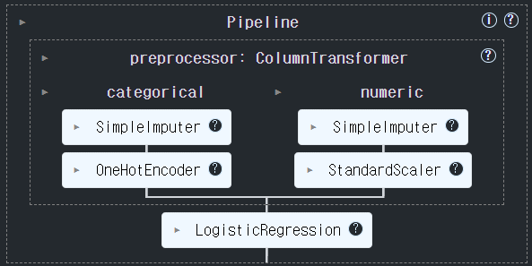
########### 컬럼별 전처리 프로세스를 pipeline으로 묶기.
### 수치형 컬럼들에 적용할 전처리 프로세스.
num_pipeline = Pipeline([
    ("imputer", SimpleImputer(strategy="mean")), # 1. 결측치 처리
    ("scaler", StandardScaler())   # 2. Feature Scaling
])
### 범주형 컬럼들에 적용할 전처리 프로세스
cate_pipeline = Pipeline([
    ("imputer", SimpleImputer(strategy="most_frequent")), 
    ("ohe", OneHotEncoder(handle_unknown='ignore'))   # handle_unknown='ignore' - 학습할 때 없었던 class는 0으로 처리.
])
preprocessor = ColumnTransformer([
    ("category", cate_pipeline, [0, 1]), 
    ("number", num_pipeline, [2, 3])
])

TODO Adult dataset

• 전처리
  • 범주형
    • 결측치는 최빈값으로 대체한다.
    • 원핫인코딩 처리한다.
  • 연속형
    • 결측치는 중앙값으로 대체한다.
    • StandardScaling을 한다.
• Model: sklearn.linear_model.LogisticRegression(max_iter=2000) 를 사용
• Pipeline을 이용해 전처리와 모델을 묶어준다.

import pandas as pd
cols = ['age', 'workclass','fnlwgt','education', 'education-num', 'marital-status', 'occupation','relationship', 'race', 'gender','capital-gain','capital-loss', 'hours-per-week','native-country', 'income']
data = pd.read_csv(
    'data/adult.data', 
    header=None,  names=cols, na_values='?', skipinitialspace=True )
categorical_columns = ['workclass','education','marital-status', 'occupation','relationship','race','gender','native-country', 'income']
numeric_columns = ['age','fnlwgt', 'education-num','capital-gain','capital-loss','hours-per-week']
categorical_columns_index = [1, 3, 5, 6, 7, 8, 9, 13]
numeric_columns_index = [0, 2, 4, 10, 11, 12]

from sklearn.model_selection import train_test_split
from sklearn.impute import SimpleImputer
from sklearn.preprocessing import OneHotEncoder, StandardScaler, LabelEncoder
from sklearn.linear_model import LogisticRegression
from sklearn.pipeline import Pipeline
from sklearn.compose import ColumnTransformer
from sklearn.metrics import accuracy_score
## X, y 분리
X = data.drop(columns='income').values  # DataFrame->ndarray
y = LabelEncoder().fit_transform(data['income']) # y->LabelEncoding (ndarray)
## Train/Test set 분리
X_train, X_test, y_train, y_test = train_test_split(X, y, stratify=y, test_size=0.25, random_state=0)
# 범주형 컬럼 전처리 파이프라인
cate_preprocessor = Pipeline([
    ("imputer", SimpleImputer(strategy="most_frequent")), 
    ("ohe", OneHotEncoder(handle_unknown="ignore"))
])
# 수치형 컬럼 전처리 파이프라인
num_preprocessor = Pipeline([
    ("imputer", SimpleImputer(strategy="median")),
    ("scaler", StandardScaler())
])
preprocessor = ColumnTransformer([
    ("categorical", cate_preprocessor, categorical_columns_index),
    ("numeric", num_preprocessor, numeric_columns_index)
])
pipeline = Pipeline([
    ("preprocessor", preprocessor),
    ("model", LogisticRegression(max_iter=2000))
])

#### GridSearchCV에 넣을 파라미터 후보 지정.
### LogisticRegression의 max_iter의 후보 : [1000, 2000, 3000]
params = {"model__max_iter":[1000, 2000, 3000]}
## preprocessor의 numeric 의 imputer (num_preprocessor) 의 strategy 후보: ["mean", "median"]
params = {"preprocssor__numeric__imputer__strategy": ["mean", "median"]}
# gs = GridSearchCV(pipeline, params, ....)
pipeline.fit(X_train, y_train)

# 검증
pred_train = pipeline.predict(X_train)
pred_test = pipeline.predict(X_test)
accuracy_score(y_train, pred_train)
accuracy_score(y_test, pred_test)

0.8527436527436527
0.8481758997666135