2022.06.21 연구실 공부(PyTorch). 'PyTorch로 시작하는 딥 러닝 입문'< 이 글은 이 책의 내용을 요약 정리한 것임.>(내 저작물이 아니고 저 위 링크에 있는 것이 원본임)
06-01 Perceptron, 06-02 XOR Problem, 06-03 BackPropagation, 06-04 Gradient Vanishing & Exploding

Summary

• Perceptron
• XOR Problem by Single-Layer Perceptron
• XOR Problem by Multi-Layer Perceptron
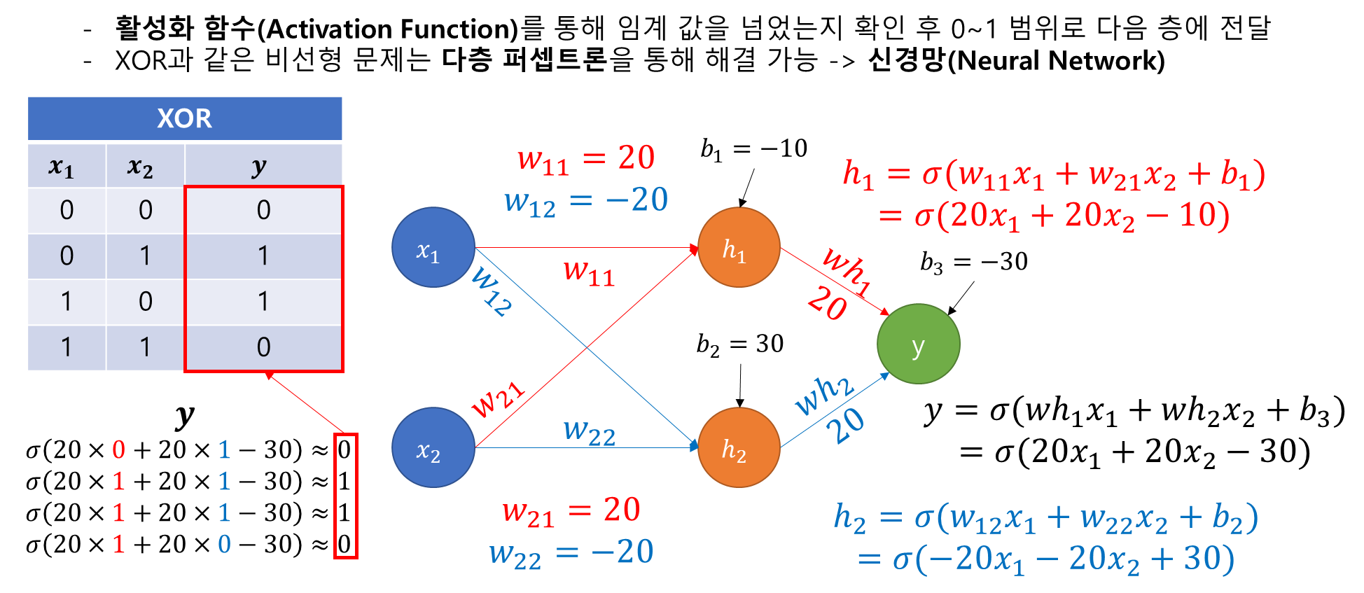
• Activation Function
• Classification by Multi-layer Perceptron
• Gradient Vanishing & Gradient Exploding

1. Perceptron

• Frank Rosenblatt가 1957년에 제안한 초기 형태의 인공 신경망
• Perceptron : 다수의 입력으로부터 하나의 결과를 내보내는 알고리즘
• 신경 세포 뉴런의 동작과 유사함
  
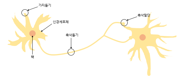
• 신경 세포 뉴런의 동작 : 가지돌기에서 신호 입력 -> 신호가 일정 수치 이상이면 축삭돌기를 통해 신호 전달
  
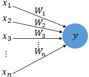
• 퍼셉트론의 동작 : 입력층(가지돌기)에서 입력 값 x(신호)를 받고 가중치 W(축삭돌기)와 함께 인공 뉴런에 전달
• 가중치가 크면 입력 값의 중요도가 크다는 것을 의미
• 입력 값과 가중치가 곱해진 값의 합이 특정 임계치를 넘기면 1, 아니면 0을 출력
• 임계치를 편향으로 넘기게 될 수도 있음 -> 이 편향도 인공신경망에서 최적 값을 찾게 됨

1-1. Single-Layer Perceptron

• 단층 퍼셉트론 : 값을 보내는 단계과 값을 받아서 출력하는 두 단계로만 이루어는 퍼셉트론
  
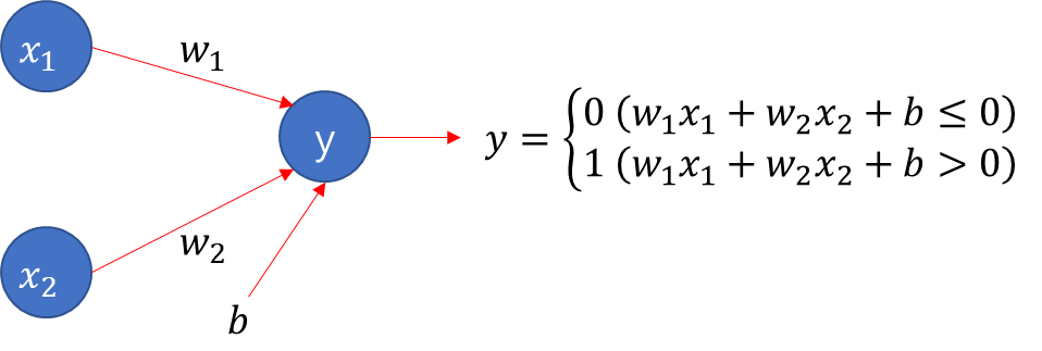
• 𝑥_1, 𝑥_2는 입력 신호, 𝑤_1, 𝑤_2는 가중치, 𝑏는 편향
• AND, NAND, OR 게이트를 쉽게 구현
• AND Gate

def AND_gate(x1, x2):
    w1=0.5
    w2=0.5
    b=-0.7
    result = x1*w1 + x2*w2 + b
    if result <= 0:
        return 0
    else:
        return 1

print(AND_gate(0, 0), AND_gate(0, 1), AND_gate(1, 0), AND_gate(1, 1))

(0, 0, 0, 1)

• NAND Gate

def NAND_gate(x1, x2):
    w1=-0.5
    w2=-0.5
    b=0.7
    result = x1*w1 + x2*w2 + b
    if result <= 0:
        return 0
    else:
        return 1

print(NAND_gate(0, 0), NAND_gate(0, 1), NAND_gate(1, 0), NAND_gate(1, 1))

(1, 1, 1, 0)

• OR Gate

def OR_gate(x1, x2):
    w1=0.6
    w2=0.6
    b=-0.5
    result = x1*w1 + x2*w2 + b
    if result <= 0:
        return 0
    else:
        return 1

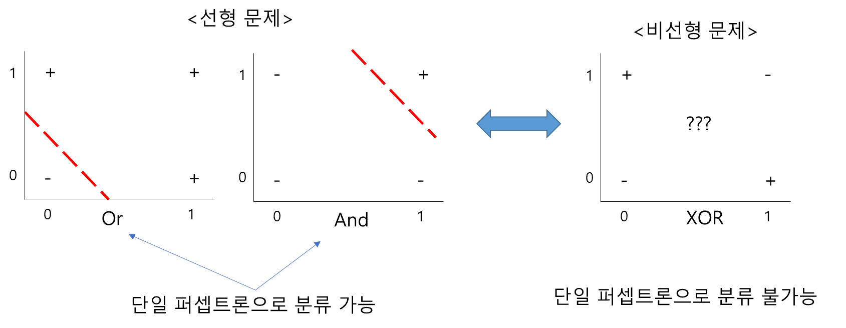
print(OR_gate(0, 0), OR_gate(0, 1), OR_gate(1, 0), OR_gate(1, 1))

(0, 1, 1, 1)

• XOR 게이트는 단층 퍼셉트론으로 표현이 불가능하다.
  

2. XOR Problem by Single Layer Perceptron

import torch
import torch.nn as nn
import torch.nn.functional as F
device = 'cuda' if torch.cuda.is_available() else 'cpu'
torch.manual_seed(777)
if device == 'cuda':
    torch.cuda.manual_seed_all(777)

X = torch.FloatTensor([[0, 0], [0, 1], [1, 0], [1, 1]]).to(device)
Y = torch.FloatTensor([[0], [1], [1], [0]]).to(device)

linear = nn.Linear(2, 1, bias=True)
sigmoid = nn.Sigmoid()
model = nn.Sequential(linear, sigmoid).to(device)

# 비용 함수와 옵티마이저 정의
criterion = torch.nn.BCELoss().to(device)
optimizer = torch.optim.SGD(model.parameters(), lr=1)
#10,001번의 에포크 수행. 0번 에포크부터 10,000번 에포크까지.
for step in range(10001): 
    optimizer.zero_grad()
    hypothesis = model(X)

    # 비용 함수
    cost = criterion(hypothesis, Y)
    cost.backward()
    optimizer.step()

    if step % 100 == 0: # 100번째 에포크마다 비용 출력
        print(step, cost.item())

• 단층 퍼셉트론으로 10001번의 에포크를 수행하고 100번마다 출력해보면
  
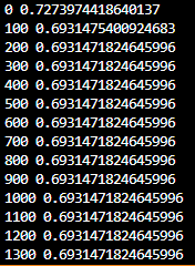
• 와 같이 0.6931471824645996 이하로 비용이 줄어들지 않음 -> 단층 퍼셉트론은 XOR 문제를 풀 수 없으므로

with torch.no_grad():
    hypothesis = model(X)
    predicted = (hypothesis > 0.5).float()
    accuracy = (predicted == Y).float().mean()
    print('모델의 출력값(Hypothesis): ', hypothesis.detach().cpu().numpy())
    print('모델의 예측값(Predicted): ', predicted.detach().cpu().numpy())
    print('실제값(Y): ', Y.cpu().numpy())
    print('정확도(Accuracy): ', accuracy.item())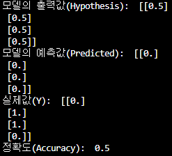

• 예측 값이 [0,0,0,0]으로 실제 값인 [0,1,1,0]을 전혀 나타내지 못하고 있다.
• 이런 비선형성 문제(XOR)는 퍼셉트론을 다층으로 쌓는것으로 해결

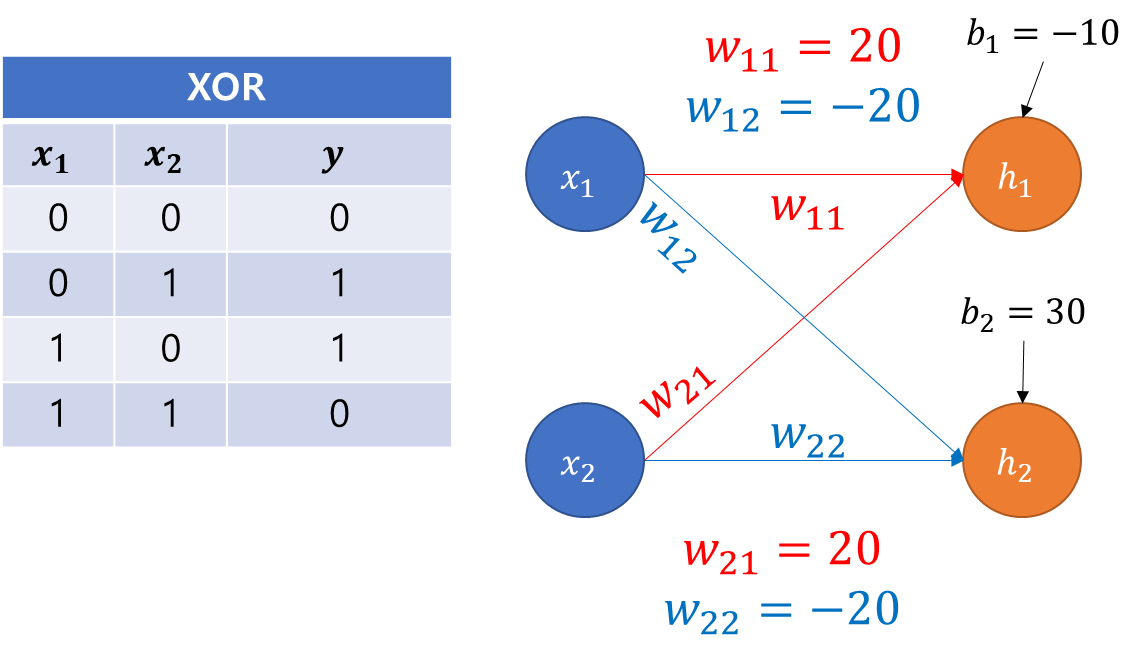
3. XOR Problem by Multi-layer Perceptron

import torch
import torch.nn as nn
device = 'cuda' if torch.cuda.is_available() else 'cpu'

# for reproducibility
torch.manual_seed(777)
if device == 'cuda':
    torch.cuda.manual_seed_all(777)

X = torch.FloatTensor([[0, 0], [0, 1], [1, 0], [1, 1]]).to(device)
Y = torch.FloatTensor([[0], [1], [1], [0]]).to(device)

model = nn.Sequential(
          nn.Linear(2, 10, bias=True), # input_layer = 2, hidden_layer1 = 10
          nn.Sigmoid(),
          nn.Linear(10, 10, bias=True), # hidden_layer1 = 10, hidden_layer2 = 10
          nn.Sigmoid(),
          nn.Linear(10, 10, bias=True), # hidden_layer2 = 10, hidden_layer3 = 10
          nn.Sigmoid(),
          nn.Linear(10, 1, bias=True), # hidden_layer3 = 10, output_layer = 1
          nn.Sigmoid()
          ).to(device)

criterion = torch.nn.BCELoss().to(device)
optimizer = torch.optim.SGD(model.parameters(), lr=1)  # modified learning rate from 0.1 to 1

for epoch in range(10001):
    optimizer.zero_grad()
    # forward 연산
    hypothesis = model(X)

    # 비용 함수
    cost = criterion(hypothesis, Y)
    cost.backward()
    optimizer.step()

    # 100의 배수에 해당되는 에포크마다 비용을 출력
    if epoch % 100 == 0:
        print(epoch, cost.item())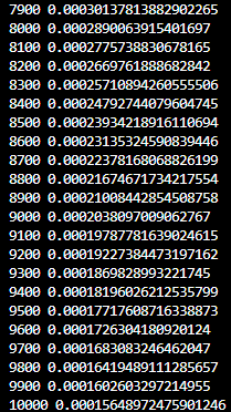

• 오차의 값이 줄어드는 것을 확인할 수 있음

with torch.no_grad():
    hypothesis = model(X)
    predicted = (hypothesis > 0.5).float()
    accuracy = (predicted == Y).float().mean()
    print('모델의 출력값(Hypothesis): ', hypothesis.detach().cpu().numpy())
    print('모델의 예측값(Predicted): ', predicted.detach().cpu().numpy())
    print('실제값(Y): ', Y.cpu().numpy())
    print('정확도(Accuracy): ', accuracy.item())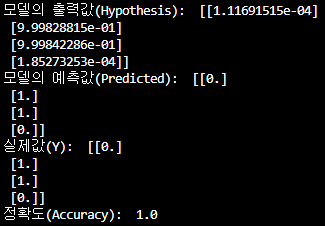

• 실제 값은 [0, 1, 1, 0]이며 예측 값은 [0, 1, 1, 0]으로 XOR문제를 해결하는 것을 알 수 있음
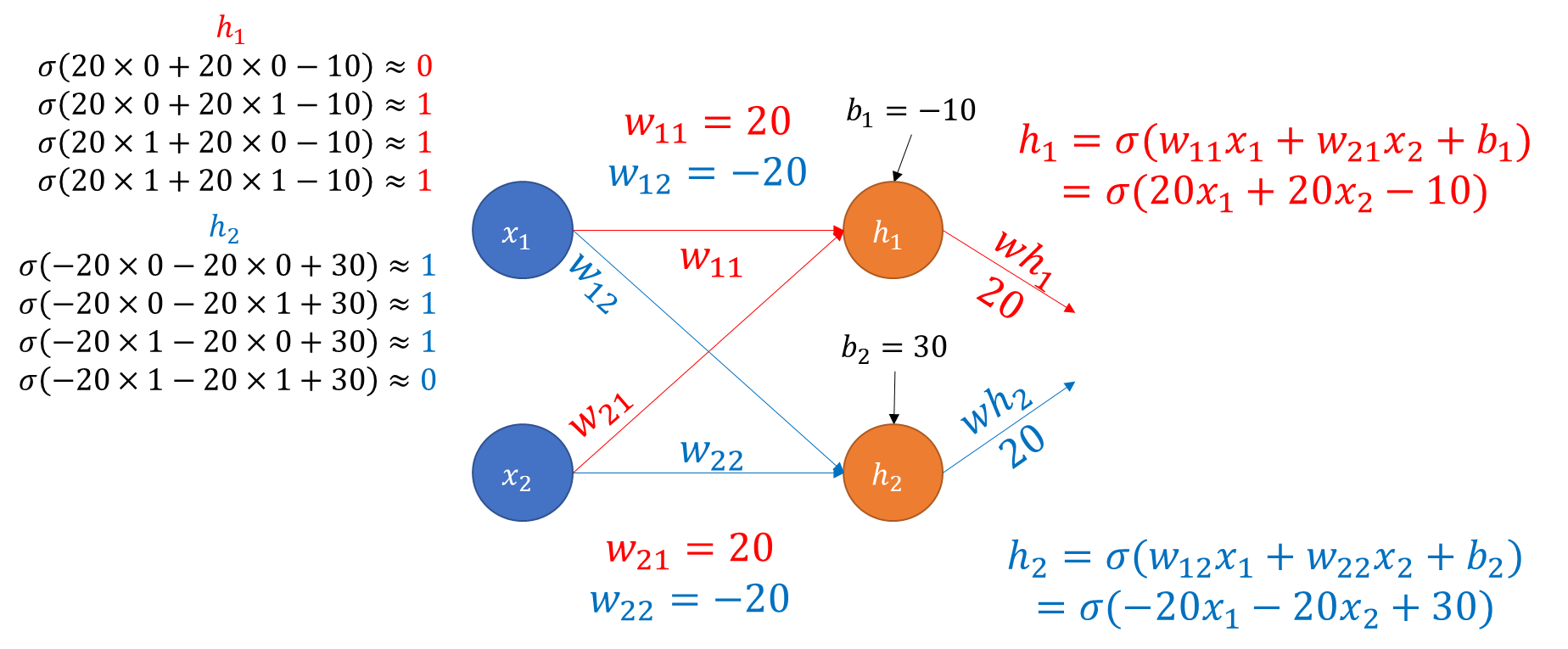
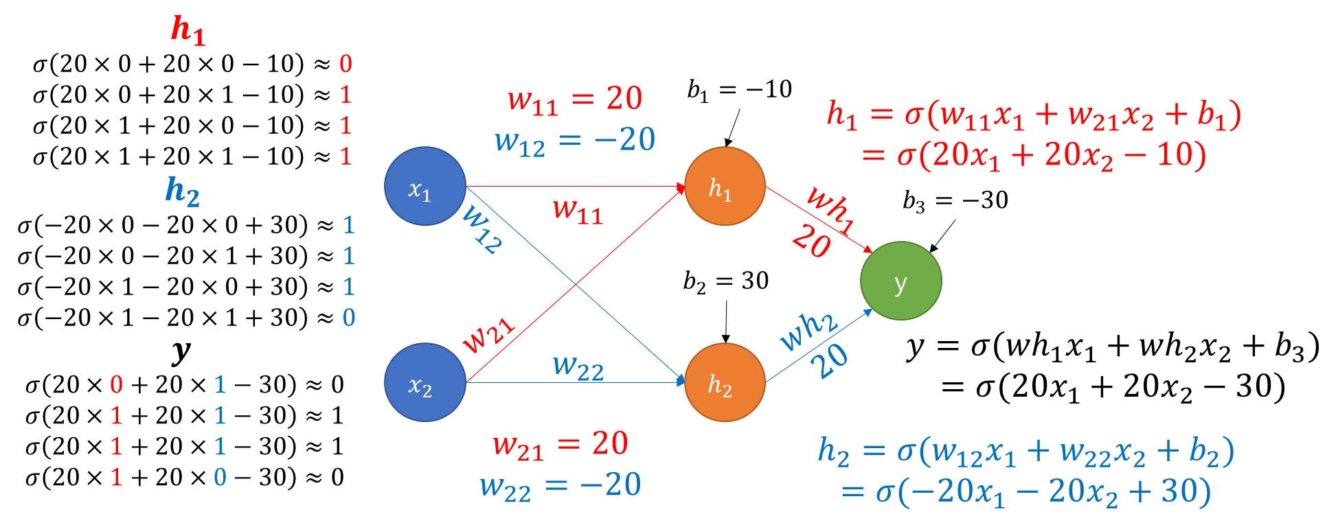
• 코드와 별개의 예시 : XOR 문제 풀이 과정 도식화
  
  
  
  

4. Activation Function

4-1. Problem of Sigmoid Function

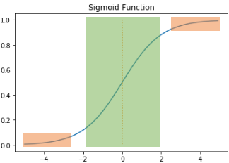
• 주황색 부분의 기울기를 계산하면 0에 가까운 아주 작은 값이 나오고 이것을 역전파 과정에서 계속 곱하게 된다면 결국, 앞에는 기울기가 잘 전달되지 않음 -> 기울기 소실(Gradient Vanishing)
  
• 이는 활성화 함수로 Sigmoid Function을 꺼리게 만드는 원인이 됨

4-2. Hyperbolic tangent function

• 입력값 -> [-1, 1] 범위의 값으로 변환

import numpy as np
import matplotlib.pyplot as plt

x = np.arange(-5.0, 5.0, 0.1) # -5.0부터 5.0까지 0.1 간격 생성
y = np.tanh(x)

plt.plot(x, y)
plt.plot([0,0],[1.0,-1.0], ':')
plt.axhline(y=0, color='orange', linestyle='--')
plt.title('Tanh Function')
plt.show()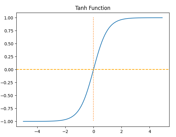

• 중심이 0이어서 반환값의 변화폭이 더 크다. -> 기울기 소실이 적다 -> 그렇다고해도 -1,1 주변에서는 확실히 기울기 소실이 발생한다.

4-3. ReLU Function

• 수식
  

def relu(x):
    return np.maximum(0, x)

x = np.arange(-5.0, 5.0, 0.1)
y = relu(x)

plt.plot(x, y)
plt.plot([0,0],[5.0,0.0], ':')
plt.title('Relu Function')
plt.show()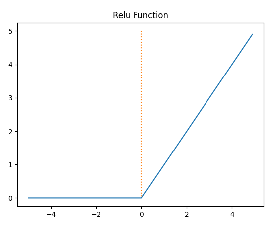

• 음수 입력시 0, 양수 입력시 그대로 반환
• 특정 양수값에 수렴하지 않아서 시그모이드보다 더 잘 변환, 연산 필요없이 그대로 전달하므로 속도도 빠름
• 입력값이 음수이면 기울기가 0이 되므로 이때는 죽은 렐루(dying ReLU)현상이 발생

4-4. Leaky ReLU

• 수식
  
• a는 하이퍼파라미터, 일반적으로는 0.01
  
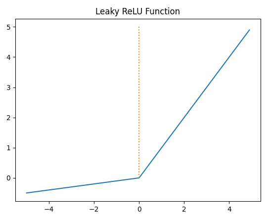
• 그래프의 기울기를 a가 조정하여 그래프가 약간 새는 모습(Leaky)을 보여준다. 이렇게하면 죽은 렐루 현상을 방지 할 수 있다.

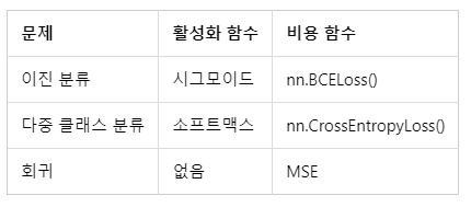
4-5. Softamx function

• 분류 문제를 로지스틱 회귀와 소프트맥스 회귀를 출력층에 적용하여 사용

x = np.arange(-5.0, 5.0, 0.1) # -5.0부터 5.0까지 0.1 간격 생성
y = np.exp(x) / np.sum(np.exp(x))

plt.plot(x, y)
plt.title('Softmax Function')
plt.show()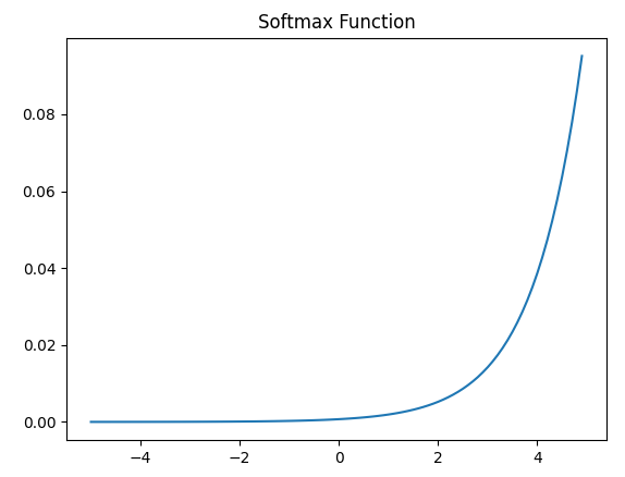

• 시그모이드 함수가 두 가지 선택지 중 하나를 고르는 이진 분류 (Binary Classification) 문제에 사용
• 소프트맥스는 세 가지 이상의 (상호 배타적인) 선택지 중 하나를 고르는 다중 클래스 분류(MultiClass Classification) 문제에 주로 사용
  

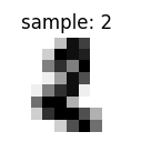
5. Classification by Multi-layer Perceptron

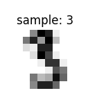
• 상위 5개 데이터 이미지 및 레이블 확인

import matplotlib.pyplot as plt # 시각화를 위한 맷플롯립
from sklearn.datasets import load_digits
digits = load_digits() # 1,979개의 이미지 데이터 로드

print(digits.images[0])

images_and_labels = list(zip(digits.images, digits.target))
for index, (image, label) in enumerate(images_and_labels[:5]): # 5개의 샘플만 출력
    plt.subplot(2, 5, index + 1)
    plt.axis('off')
    plt.imshow(image, cmap=plt.cm.gray_r, interpolation='nearest')
    plt.title('sample: %i' % label)
    #plt.show()

• 퍼셉트론 분류기 코드

import matplotlib.pyplot as plt # 시각화를 위한 맷플롯립
from sklearn.datasets import load_digits
digits = load_digits() # 1,979개의 이미지 데이터 로드

print(digits.images[0])

for i in range(5):
  print(i,'번 인덱스 샘플의 레이블 : ',digits.target[i])

X = digits.data # 이미지. 즉, 특성 행렬
Y = digits.target # 각 이미지에 대한 레이블

import torch
import torch.nn as nn
from torch import optim
model = nn.Sequential(
    nn.Linear(64, 32), # input_layer = 64, hidden_layer1 = 32
    nn.ReLU(),
    nn.Linear(32, 16), # hidden_layer2 = 32, hidden_layer3 = 16
    nn.ReLU(),
    nn.Linear(16, 10) # hidden_layer3 = 16, output_layer = 10
)
X = torch.tensor(X, dtype=torch.float32)
Y = torch.tensor(Y, dtype=torch.int64)
loss_fn = nn.CrossEntropyLoss() # 이 비용 함수는 소프트맥스 함수를 포함하고 있음.
optimizer = optim.Adam(model.parameters())
losses = []
for epoch in range(100):
  optimizer.zero_grad()
  y_pred = model(X) # forwar 연산
  loss = loss_fn(y_pred, Y)
  loss.backward()
  optimizer.step()

  if epoch % 10 == 0:
    print('Epoch {:4d}/{} Cost: {:.6f}'.format(
            epoch, 100, loss.item()
        ))

  losses.append(loss.item())
plt.plot(losses)
plt.show()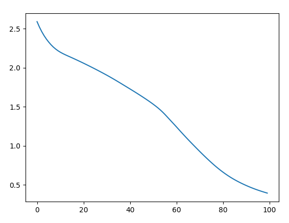

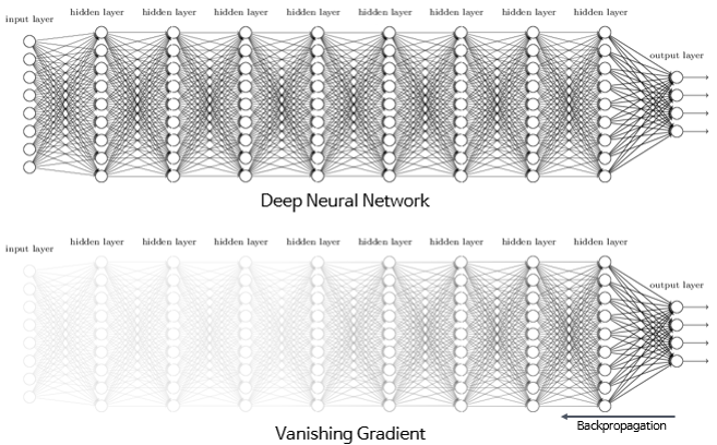
6. Gradient Vanishing & Gradient Exploding

• 기울기 소실(Gradient Vanishing) : 깊은 신경망을 역전파 중에 입력층으로 갈수록 기울기가 점차 작아져 결국 가중치 업데이트가 제대로 되지 않는 현상
• 기울기 폭주(Gradient Exploding) : 기울기가 점차 커지더니 가중치들이 비정상적으로 큰 값이 되면서 결국 발산되는 현상

6-1. ReLU와 ReLU의 변형 사용

• 시그모이드 함수의 출력값이 0 또는 1에 수렴하면서 기울기가 0에 가까워지므로 기울기 소실이 일어나기 좋음 -> ReLU나 ReLU의 변형 함수와 같은 Leaky ReLU를 사용
• 은닉층에서는 시그모이드 함수를 사용하지 말 것
• Leaky ReLU를 사용하면 모든 입력값에 대해서 기울기가 0에 수렴하지 않아 죽은 ReLU 문제를 해결

6-2. 세이비어 초기화(Xavier Initialization)

• 이전 층의 뉴런 개수를 n_in, 다음 층의 뉴런 개수를 n_out라 가정할 때
• 균등 분포(Uniform Distribution)의 경우
  
  
• 정규 분포(Normal distribution)의 경우
  
• 세이비어 초기화는 특정 층이 너무 주목받거나 너무 뒤쳐지는 것을 방지 -> S자형 함수(시그모이드 등)과는 좋은 조합이 되지만, ReLU와는 별로 좋은 조합이 아님

6-3. He 초기화(He initialization)

• 세이비어 초기화와 다르게 다음 층의 뉴런의 수를 반영하지 않음
• 균등 분포의 경우
  
• 정규 분포의 경우
  
• ReLU 계열 함수를 사용할 경우에는 He 초기화 방법이 효율적 -> ReLU + He 초기화 방법이 좀 더 보편적임

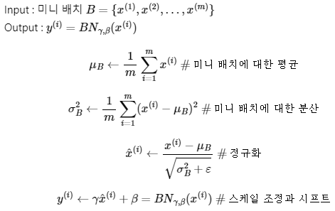
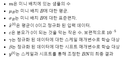
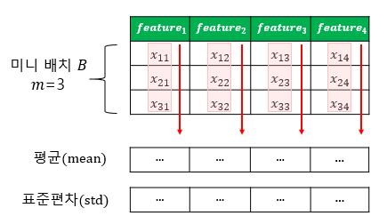
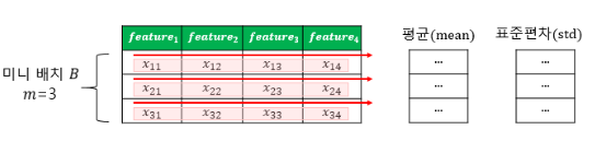
6-4. 배치 정규화(Batch Normalization)와 층 정규화(Layer Normalization)

• 한 번에 들어오는 배치 단위로 정규화하는 것 -> 학습 시 배치 단위의 평균과 분산들을 차례대로 받아 이동 평균과 이동 분산을 저장해놓았다가 테스트 할 때는 해당 배치의 평균과 분산을 구하지 않고 구해놓았던 평균과 분산으로 정규화
  
  
• 시그모이드 함수나 하이퍼볼릭탄젠트 함수를 사용하더라도 기울기 소실 문제가 크게 개선
• 가중치 초기화에 훨씬 덜 민감
• 훨씬 큰 학습률을 사용할 수 있어 학습 속도를 개선
• 단점 : 미니 배치 크기에 의존적, RNN에 적용하기 어려움
• 배치 정규화 시각화
  
• 층 정규화 시각화
  

출처 : 'PyTorch로 시작하는 딥 러닝 입문' <이 책의 내용을 요약 정리한 것임.>