개요
- 전이학습(Transfer Learning)을 적용
- 특히, VGG16이라는 잘 훈련된 CNN 모델의 특징 추출기를 활용하여
적은 학습 데이터로도 높은 성능 - 이번 글에서는 VGG16 개념 설명과 함께,
사전학습된 weight를 활용한 이미지 분류 실습을 정리
1. 전이학습이란?
- 전이학습은 다른 대규모 데이터셋에서 미리 학습된 모델의 지식을 재사용
- CNN의 하위 층은 엣지, 색상, 패턴 등 일반적인 시각 특징을 잘 추출
- 이러한 특성을 그대로 가져와 새로운 데이터에 적용하면
적은 양의 데이터로도 높은 정확도 획득
2. VGG16이란?
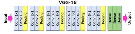
- VGG16은 2014년 ILSVRC 대회에서 우수한 성능을 보인 CNN 구조임
- 16개의 계층(Conv + FC)으로 구성됨
- 단순하면서도 강력한 구조로 이미지 분류에서 널리 사용됨
- ImageNet(1천만 개 이상 이미지, 1,000개 클래스)으로 학습된 weight 제공됨
- 여기서는 top layer (fully connected classifier)를 제거하고
Conv layer만 사용하여 특징 추출기로 활용함
3. 사전학습된 VGG16 로드
from tensorflow.keras.applications.vgg16 import VGG16

conv_base = VGG16(weights='imagenet',  # ImageNet으로 학습된 가중치 사용
                  include_top=False,   # 최상단 분류기 제거
                  input_shape=(150, 150, 3))  # 입력 이미지 크기 지정

conv_base.summary()
Model: "vgg16"
┏━━━━━━━━━━━━━━━━━━━━━━━━━━━━━━━━━━━━━━┳━━━━━━━━━━━━━━━━━━━━━━━━━━━━━┳━━━━━━━━━━━━━━━━━┓
┃ Layer (type) ┃ Output Shape ┃ Param # ┃
┡━━━━━━━━━━━━━━━━━━━━━━━━━━━━━━━━━━━━━━╇━━━━━━━━━━━━━━━━━━━━━━━━━━━━━╇━━━━━━━━━━━━━━━━━┩
│ input_layer (InputLayer) │ (None, 150, 150, 3) │ 0 │
├──────────────────────────────────────┼─────────────────────────────┼─────────────────┤
│ block1_conv1 (Conv2D) │ (None, 150, 150, 64) │ 1,792 │
├──────────────────────────────────────┼─────────────────────────────┼─────────────────┤
│ block1_conv2 (Conv2D) │ (None, 150, 150, 64) │ 36,928 │
├──────────────────────────────────────┼─────────────────────────────┼─────────────────┤
│ block1_pool (MaxPooling2D) │ (None, 75, 75, 64) │ 0 │
├──────────────────────────────────────┼─────────────────────────────┼─────────────────┤
│ block2_conv1 (Conv2D) │ (None, 75, 75, 128) │ 73,856 │
├──────────────────────────────────────┼─────────────────────────────┼─────────────────┤
│ block2_conv2 (Conv2D) │ (None, 75, 75, 128) │ 147,584 │
├──────────────────────────────────────┼─────────────────────────────┼─────────────────┤
│ block2_pool (MaxPooling2D) │ (None, 37, 37, 128) │ 0 │
├──────────────────────────────────────┼─────────────────────────────┼─────────────────┤
│ block3_conv1 (Conv2D) │ (None, 37, 37, 256) │ 295,168 │
├──────────────────────────────────────┼─────────────────────────────┼─────────────────┤
│ block3_conv2 (Conv2D) │ (None, 37, 37, 256) │ 590,080 │
├──────────────────────────────────────┼─────────────────────────────┼─────────────────┤
│ block3_conv3 (Conv2D) │ (None, 37, 37, 256) │ 590,080 │
├──────────────────────────────────────┼─────────────────────────────┼─────────────────┤
│ block3_pool (MaxPooling2D) │ (None, 18, 18, 256) │ 0 │
├──────────────────────────────────────┼─────────────────────────────┼─────────────────┤
│ block4_conv1 (Conv2D) │ (None, 18, 18, 512) │ 1,180,160 │
├──────────────────────────────────────┼─────────────────────────────┼─────────────────┤
│ block4_conv2 (Conv2D) │ (None, 18, 18, 512) │ 2,359,808 │
├──────────────────────────────────────┼─────────────────────────────┼─────────────────┤
│ block4_conv3 (Conv2D) │ (None, 18, 18, 512) │ 2,359,808 │
├──────────────────────────────────────┼─────────────────────────────┼─────────────────┤
│ block4_pool (MaxPooling2D) │ (None, 9, 9, 512) │ 0 │
├──────────────────────────────────────┼─────────────────────────────┼─────────────────┤
│ block5_conv1 (Conv2D) │ (None, 9, 9, 512) │ 2,359,808 │
├──────────────────────────────────────┼─────────────────────────────┼─────────────────┤
│ block5_conv2 (Conv2D) │ (None, 9, 9, 512) │ 2,359,808 │
├──────────────────────────────────────┼─────────────────────────────┼─────────────────┤
│ block5_conv3 (Conv2D) │ (None, 9, 9, 512) │ 2,359,808 │
├──────────────────────────────────────┼─────────────────────────────┼─────────────────┤
│ block5_pool (MaxPooling2D) │ (None, 4, 4, 512) │ 0 │
└──────────────────────────────────────┴─────────────────────────────┴─────────────────┘
Total params: 14,714,688 (56.13 MB)
Trainable params: 14,714,688 (56.13 MB)
Non-trainable params: 0 (0.00 B)include_top=False설정으로 FC layer 제거- 최종 출력은
(4, 4, 512)크기의 feature map 생성 - 이 feature map을 flatten하여 완전 연결층에 전달
4. 이미지에서 특징 추출
conv_base로부터 이미지별 특징을 추출하여 Dense 레이어 학습에 활용- 학습 대상: 2,000개(train), 1,000개(validation), 1,000개(test)
import numpy as np
from tensorflow.keras.preprocessing.image import ImageDataGenerator

datagen = ImageDataGenerator(rescale=1./255)
batch_size = 20

def extract_features(directory, sample_count):
    features = np.zeros((sample_count, 4, 4, 512))
    labels = np.zeros(sample_count)
    generator = datagen.flow_from_directory(
        directory,
        target_size=(150, 150),
        batch_size=batch_size,
        class_mode='binary')
    i = 0
    for inputs_batch, labels_batch in generator:
        features_batch = conv_base.predict(inputs_batch)
        features[i * batch_size : (i + 1) * batch_size] = features_batch
        labels[i * batch_size : (i + 1) * batch_size] = labels_batch
        i += 1
        if i * batch_size >= sample_count:
            break
    return features, labels

train_features, train_labels = extract_features(train_dir, 2000)
validation_features, validation_labels = extract_features(validation_dir, 1000)
test_features, test_labels = extract_features(test_dir, 1000)

train_features = np.reshape(train_features, (2000, 4 * 4 * 512))
validation_features = np.reshape(validation_features, (1000, 4 * 4 * 512))
test_features = np.reshape(test_features, (1000, 4 * 4 * 512))
5. 완전 연결층 구성 및 학습
conv_base로부터 추출한 특징 벡터를 Dense 레이어에 넣고 학습- 이 단계에서는 Conv 레이어는 고정되고, FC 레이어만 학습
from keras import models, layers
from tensorflow.keras.optimizers import RMSprop

model = models.Sequential()
model.add(layers.Dense(256, activation='relu', input_dim=4 * 4 * 512))
model.add(layers.Dropout(0.5))
model.add(layers.Dense(1, activation='sigmoid'))

model.compile(loss='binary_crossentropy',
              optimizer=RMSprop(learning_rate=2e-5),
              metrics=['acc'])

history = model.fit(train_features, train_labels,
                    epochs=100,
                    batch_size=20,
validation_data=(validation_features, validation_labels))- Dropout 적용으로 과적합 방지
- learning rate를 낮게 설정하여 안정적인 학습 유도
6. 학습 결과 시각화
- 학습 정확도와 검증 정확도를 시각화하여 모델 성능 확인
import matplotlib.pyplot as plt

acc = history.history['acc']
val_acc = history.history['val_acc']
loss = history.history['loss']
val_loss = history.history['val_loss']

epochs = range(1, len(acc)+1)

plt.plot(epochs, acc, 'bo', label='Training acc')
plt.plot(epochs, val_acc, 'b', label='Validation acc')
plt.title('Training and validation accuracy')
plt.legend()

plt.figure()
plt.plot(epochs, loss, 'bo', label='Training loss')
plt.plot(epochs, val_loss, 'b', label='Validation loss')
plt.title('Training and validation loss')
plt.legend()

plt.show()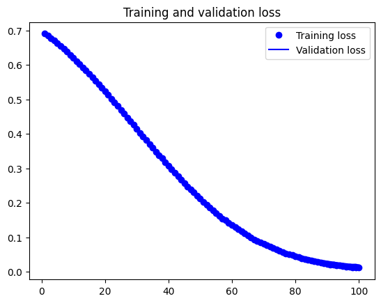
- 훈련 정확도와 검증 정확도가 일정하게 상승하며 과적합이 크게 줄어든 모습 보임
- 사전학습된 weight 덕분에 안정적인 학습 결과 얻음
마무리
- 사전학습된 VGG16 모델을 활용하여 작은 데이터셋에서도 높은 성능을 확보
- 이 실험은 전이학습의 효과를 잘 보여주는 대표적인 예시
- 특히 Feature Extraction만으로도 일반적인 CNN보다 훨씬 좋은 성능 달성
- 실제 현업에서도 데이터가 부족하거나 빠른 실험이 필요한 경우 전이학습을 많이 사용

gpt로 다시 배우는 개발