[ICLR2018]Enhancing The Reliability of Out-Of-Disribution Image Detection In Neural Networks - [2022.06.28]

ABSTRACT

본 논문에서는 ODIN이라는 쉽고 효율적인 방법을 제안한다. 이 방법은 pre-trained된 neural network의 어떤 변화도 필요로 하지 않는다. 이 방법은 temperature scaling과 입력 이미지에 small perturbations을 더해줌으로써 in- and out-of-distribution사이의 softmax score를 더 효과적으로 분리할 수 있다.

INTRODUCTION

딥러닝이 발전함에 있어서 여러 문제들이 있지만, 이 논문에서 다루고자 하는 문제는 처음보는 입력을 어떻게 처리할 것인지에 대한 것이다. 딥러닝이 신뢰할 수 있을만한 수준이 되기 위해서는 처음보는 입력(Out-of-distribution)에 대해서 불확실성을 가질 수 있는 것이 중요하다.

Hendrycks & Gimpel은 이러한 문제(Detecting out-of-distribution)를 해결하기 위한 baseline을 제시했는데, 이 때, 모델의 재훈련 없이 이를 가능케 했다. 그 방법은 잘 훈련된 neural-networks가 in-distribution 입력들을 out-of-distribution보다 더 높은 softmax scores를 갖도록 만들어 분리하는 것이었다.

그리고 이 논문(ODIN)에서는 여기에 덧붙여, softmax function에서 temperature scaling을 적용하고 작은 조작가능한 perturbations를 입력에 더해주는 것으로 in- and out-of-distribution softmax score의 차이를 더욱 크게 만들었다.

PROBLEM STATEMENT

$P_\mathbf{x}$ : in-distribution
$Q_\mathbf{x}$ : out-distribution

$\mathbb{P}_{\mathbf{x}\times{\mathbf{z}}}$
$\mathbb{P}_\mathbf{x|z=0}=P_\mathbf{x}$
$\mathbb{P}_\mathbf{x|z=1}=Q_\mathbf{x}$

Given an image $X$ drawn from the mixture distribution $\mathbb{P}_\mathbf{x\times{z}}$, can we distinguish whether the image is from in-distribution $P_\mathbf{x}$ or not?

Temperature scaling

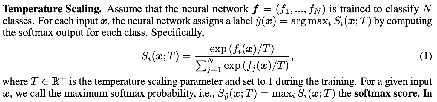
이러한 temperature scaling을 통해 저자들은 in- and out-of-distribution 이미지들 사이의 the softmax scores를 잘 분리하였다. 이는 out-of-distribution 탐지를 효과적으로 만들어 준다.

images, _ = data
        
inputs = Variable(images.cuda(CUDA_DEVICE), requires_grad = True)
outputs = net1(inputs)
# Calculating the confidence of the output, no perturbation added here, no temperature scaling used
nnOutputs = outputs.data.cpu()
nnOutputs = nnOutputs.numpy()
nnOutputs = nnOutputs[0]
nnOutputs = nnOutputs - np.max(nnOutputs)
nnOutputs = np.exp(nnOutputs)/np.sum(np.exp(nnOutputs))

여기서 중간 부분에 정규화가 다음과 같이 들어간다.

nnOutputs - np.max(nnOutputs)

이 식의 의미는, nnOutputs의 경우 logit 값으로 어떤 값이 나오는지는 모르겠지만, 이 값이 매우 크게될 경우, softmax를 구하는 과정에서 np.exp(nnOutputs)값이 무한대($\infty$)가 될 수 있다. 따라서, softmax 함수의 property느 유지하되, 위와 같은 문제가 발생하지 않기 위해서, max 값으로 빼줌으로써 정규화를 진행한다.

# Using temperature scaling
outputs = outputs / temper # ????
	
# Calculating the perturbation we need to add, that is,
# the sign of gradient of cross entropy loss w.r.t. input
maxIndexTemp = np.argmax(nnOutputs)
labels = Variable(torch.LongTensor([maxIndexTemp]).cuda(CUDA_DEVICE))
loss = criterion(outputs, labels)
loss.backward()

    images, _ = data
    
    inputs = Variable(images.cuda(CUDA_DEVICE), requires_grad = True)
    outputs = net1(inputs) # logit 값

    print('logit : ', outputs )
    nnOutputs = outputs.data.cpu()
    nnOutputs = nnOutputs.numpy()
    nnOutputs = nnOutputs[0]
    print('logit 1 array : ', nnOutputs)
    nnOutputs_regual = nnOutputs - np.max(nnOutputs)
    print('regularized nnOutputs : ', nnOutputs_regual)
    nnOutputs = np.exp(nnOutputs) / np.sum(np.exp(nnOutputs))
    print('normal nn : ', nnOutputs)
    nnOutputs_regual = np.exp(nnOutputs_regual) / np.sum(np.exp(nnOutputs_regual))
    print('regul nn : ', nnOutputs_regual)
    ## 결과 값은 같음.
    
    outputs_div_tem = outputs / 1000
    tem = outputs_div_tem.data.cpu()
    tem = tem.numpy()
    tem = tem[0]
    print('ori output: ',outputs)
    print('tem_output: ',outputs_div_tem)

    print('tem_crossentropy : ', np.exp(tem) / np.sum(np.exp(tem)))

    maxIndexTemp = np.argmax(nnOutputs_regual)
    print('label_index : ', maxIndexTemp)
    labels = Variable(torch.LongTensor([maxIndexTemp]).cuda(CUDA_DEVICE))
    print('label : ', labels)
    loss = criterion(outputs_div_tem, labels)
    loss_ori = criterion(outputs, labels)
    print('loss : ', loss)
    print('loss_ori : ', loss_ori)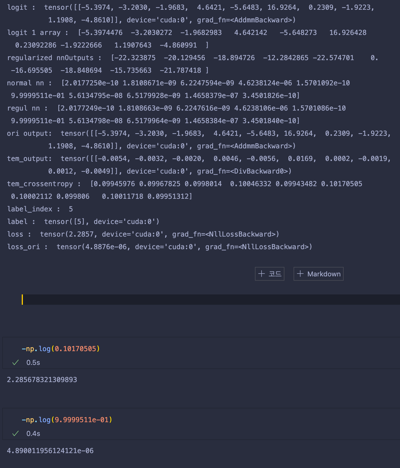

logit과 위 수식들에 대해 간략하게 출력해봤다.

위 그림을 보면 tem_output은 기존 ori output에서 1000을 나눈 값으로, 기존 logit 값보다 1000배 작아진 모습이다.

이렇게 만든 까닭은, 이를 softmax probability로 만들어 주었을 때 그 이유가 있다.

normal nn의 결과값을 보면, 5번째 인덱스의 값에서 9.9999511e-01결과값 1에 거의 수렴하는 모습을 볼 수 있다.

이는, 아무런 처리도 하지 않은 logit값이 exp() 함수에 입력으로 들어갈 경우, 아주 작은 값이더라도 매우 빠른 속도로 증가하기 때문에, 기존에 학습된 모델들은 매우 높은값의 confidence를 가지는 softmax probability를 출력한다.

이를 해결하기 위해서 temperature를 이용해 logit값들을 나눴고, outputs/tem을 softmax probability로 사용하여 기존의 softmax probability보다 확연히 confidence값이 낮아지고, uniform해 진 것을 확인할 수 있다.(근데 이건 너무 uniform한 게 아닌가.. ? 여튼)

Input Preprocessing (adding perturbation)

이제 여기에 Input Preprocessing으로 small perturbations를 집어넣어보자.

일반적으로 adversarial attack에서 사용되는 adding small perturbation기법은, model을 regularize할 때도 종종 사용한다. (많이 사용되지는 않는듯)

        loss.backward()
        
        # Normalizing the gradient to binary in {0, 1}
        gradient =  torch.ge(inputs.grad.data, 0)
        gradient = (gradient.float() - 0.5) * 2
        # Normalizing the gradient to the same space of image
        gradient[0][0] = (gradient[0][0] )/(63.0/255.0)
        gradient[0][1] = (gradient[0][1] )/(62.1/255.0)
        gradient[0][2] = (gradient[0][2])/(66.7/255.0)
        # Adding small perturbations to images
        tempInputs = torch.add(inputs.data,  -noiseMagnitude1, gradient)
        outputs = net1(Variable(tempInputs))

loss.backward()은 모델의 모든 학습 가능한 매개변수의 변화도(gradient)를 계산하는 함수입니다.

이 함수를 실행시키고 나면, inputs에 대한 grad값이 발생하고, torch.ge를 통해 inputs.grad.data가 0보다 큰 경우만 gradient로 저장해줍니다. 그리고 나서 gradient.float() 으로 float로 만든 뒤 Normalizing을 진행한다. 이후 torch.add()를 통해 -noiseMagnitude1을 gradient에 곱해주면서, 식 2번을 만족시킨다.

Out-of-distribution Detector

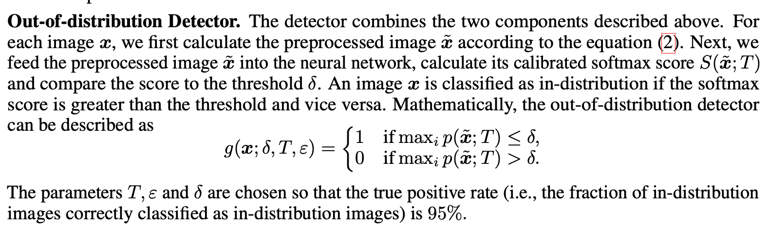
논문의 저자는 굉장히 심플하게 Out-of-distribution을 탐지한다. 각 이미지 $x$에 대해서, 먼저 전처리된 이미지인(add perturbation) $x'$를 구한다. 그러고나서, 전처리된 이미지 $x'$를 학습된 neural network에 넣고 calibrated softmax score $S(x';T)$를 한 뒤, threshold $\delta$를 가지고 socore들을 비교한다. 이미지 $x$의 softmax score가 threshold $\delta$보다 크다면, in-distribution, 아니면 out-of-distribution으로 한다는 말이다. 이 때, 저자들은 TPR이 95일때의 Out-of-distribution FPR을 구하였다.

ROC Curves

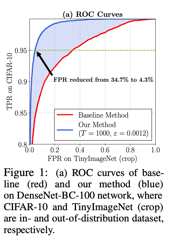
위 그림에서 초록색 점선은 CIFAR-10의 TPR이 0.95인 경우의 Out-of-distribution의 FPR을 나타낸다. 보는 것과 같이, 기존 베이스라인 모델은 TPR 0.95의 경우 약 약 34.7%의 FPR을 보이지만, Temperatur scalling과 perturbation을 진행한 경우 4.3%로 매우 적은 FPR을 보이는 것으로 확인된다.

Conclusions

이 논문에서는, 간단하고 효과적인 out-of-distribution 방법에 대해 제안한다. 이 방법은 이미 학습된 네트워크를 재학습할 필요가 없으며, 기존 베이스라인 모델에서 크게 향상된 결과를 보인다. 논문의 저자들은 경험적으로 이 방법이 파라미터 세팅값에 따라 다르게 되는 것을 분석했으며, 미래의 작업에 이러한 방법론이 이미지 뿐만 아니라 speech recognition 그리고 NLP에서 사용될 수 있을 것이다.