[부스트캠프 AI Tech] 3주차 Day 2

Mattaaa·2022년 2월 4일

U stage 부스트캠프 AI Tech

[부스트캠프 AI Tech]

목록 보기

11/23

오늘 학습 내용

1. Seaborn

Matplotlib 기반 통계 시각화 Library 이며, 다양한 커스텀 및 쉬운 문법, 깔끔한 디자인이 특징.
시각화의 목적과 방법에 따른 API 분류
- Categorical API
- Distribution API
- Realational API
- Regression API
- Multiples API
- Theme API

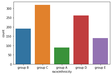
Categorical API

Countplot

Seaborn의 Categorical API에서 대표적인 시각화 Method
sns.countplot(x='column', data = datas, hue='split_column', order=sorted())
hue는 색으로 데이터 구분 기준을 정하는데 사용.

order로 순서 명시 가능.

통계량

Count : Data 수
Mean : 평균
Std : 표준편차
사분위수 : 데이터를 4등분한 관측값 (25%, 50% 75%)

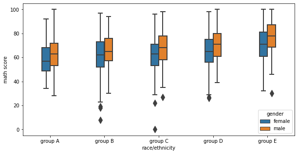
Box Plot

중간의 사각형은 각각 25%, medium, 50% 값을 의미

사각형의 사이(25%~75%) 를 IQR(Interquartile Range) 라 한다.

25% 와 75% 값에 각각 -1.5, 1.5 배한 값을 whisker(경계선)으로 정하고, 범위 밖의 값을 Outlier라 한다.
fig, ax = plt.subplots(1,1, figsize=(10, 5))
sns.boxplot(x='column1', y='column2', data=datas,
            hue='split_column', 
            order=sorted(),
            width=0.3,
            linewidth=2,
            fliersize=10, #outlier 점의 크기
            ax=ax)
plt.show()
Violin Plot

Box Plot에 비해, 실제 분포를 표현하기에 적합

IQR을 표현하는 방법이 여러가지이다.

bw : 분포 표현의 구체화 수치

cut : 경계값 설정

inner : 내부 IQR 표현 방식
fig, ax = plt.subplots(1,1, figsize=(12, 5))
sns.violinplot(x='column1', data=datas, ax=ax,
               bw=0.1,
               cut=0,
               inner='quartile'
              )
plt.show()

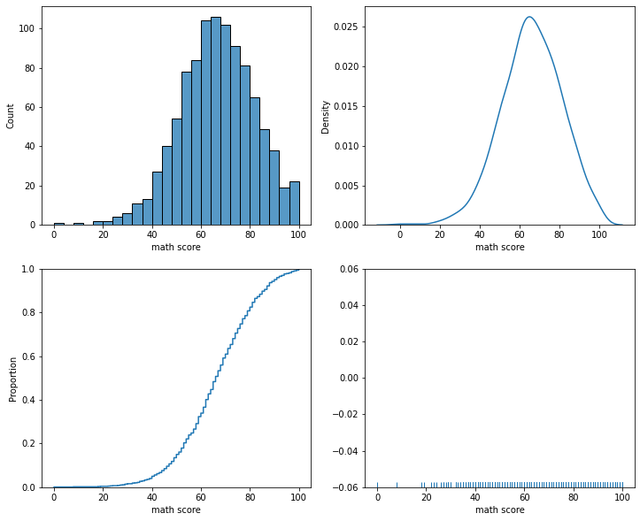
Distribution API

hisplot : 히스토그램
kdeplot : Kernel Densitiy Estimate
ecdfplot : 누적 밀도 함수
rugplot : 선을 사용한 밀도함수

fig, axes = plt.subplots(2,2, figsize=(12, 10))
axes = axes.flatten()
sns.histplot(x='math score', data=student, ax=axes[0])
sns.kdeplot(x='math score', data=student, ax=axes[1]) #곡선 보간
sns.ecdfplot(x='math score', data=student, ax=axes[2])
sns.rugplot(x='math score', data=student, ax=axes[3])

Relation & Regression

Scatter Plot

style, hue, size 설정 가능

fig, ax = plt.subplots(figsize=(7, 7))
sns.scatterplot(x='column1', y='column2', data=data,
                hue='race/ethnicity')

Line Plot

fig, ax = plt.subplots(1, 1,figsize=(12, 7))
sns.lineplot(x='year', y='Jan',data=flights_wide, ax=ax)

Regplot

Scatter Plot에 회귀선을 추가한 Plot이다.
order 사용 시, 2차원의 회귀선을 사용 할 수 있으며, log 선 또한 사용 가능.

fig, ax = plt.subplots(figsize=(7, 7))
sns.regplot(x='math score', y='reading score', data=student)

fig, ax = plt.subplots(figsize=(7, 7))
sns.regplot(x='reading score', y='writing score', data=student,
            logx=True)

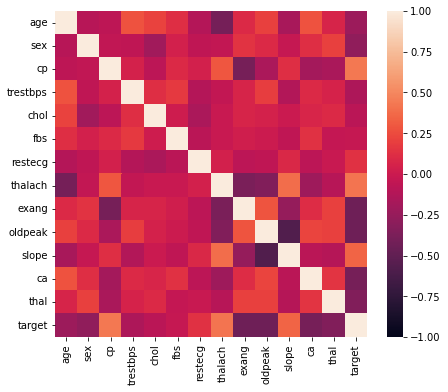
Matrix Plots

Heatmap

상관관계(Correlation) 시각화에 대표적으로 사용된다.
vmin과 vmax를 통한 범위 조정.

fig, ax = plt.subplots(1,1 ,figsize=(7, 6))
sns.heatmap(heart.corr(), ax=ax,
           vmin=-1, vmax=1)

annot, fmt 을 사용하여 실제 값에 들어갈 내용 삽입

fig, ax = plt.subplots(1,1 ,figsize=(10, 9))
sns.heatmap(heart.corr(), ax=ax,
           vmin=-1, vmax=1, center=0,
            cmap='coolwarm',
            annot=True, fmt='.2f')