기초부터 차근차근 다져가는 것이 제일 중요하다고 생각하지만 막상 익숙한 내용이면 스킵하기에 바빴다. 그래서 이번에는 마음가짐을 다르게 해서 접근하려고 한다.
데이터 사이언스 프로젝트를 단계별로 접근하는 notebook이 있어서 읽어보려고 한다.
Titanic Data Science Solutions : Data Science Solutions 라는 책을 토대로 작성했다고 함.
Workflow stages
- Question or problem definition.
- Acquire training and testing data.
- Wrangle, prepare, cleanse the data.
- Analyze, identify patterns, and explore the data.
- Model, predict and solve the problem.
- Visualize, report, and present the problem solving steps and finale solution.
- Supply or submit the results.
- 여러가지 단계를 합칠 수 있다. 시각화된 데이터를 분석.
- 위 순서보다 일찍 실행할 수 있다. wrangling 전후로 분석.
- 하나의 단계를 여러번 실행. 시각화 단계는 여러번 실행해야 함.
- 여러 단계를 한꺼번에 하지 않아도 된다. competition에 대한 서비스 가능하거나 생산 가능한 데이터셋을 제공하지 않아도 된다.
Question and problem definition
캐글과 같은 competition 사이트는 풀어야 할 문제나 물어볼 문제를 정의해준다. 데이터 사이언스 모델을 학습시키는 데이터도 제공하고 모델을 테스트할 테스트셋도 제공해준다.
Knowing from a training set of samples listing passengers who survived or did not survive the Titanic disaster, can our model determine based on a given test dataset not containing the survival information, if these passengers in the test dataset survived or not.
Workflow goals
7가지의 주된 목표가 있음!!
- Classifying
- 데이터를 분류하고 카테고리별로 나누기.
- Correlating
- 어떤 문제는 training dataset 내에서 사용 가능한 features를 기반으로 해결할 수 있음
- dataset 안에 있는 어떤 features가 문제 해결에 적절한지, 해결 방법과 feature 사이에 연관성은 어떤지.
- Converting
- 모델링하는 단계에서, 데이터를 준비하는 것이 필요하다.
- 모델 알고리즘을 선택하는 것에 따라서 모든 features을 수치적으로 비슷한 값으로 바꿔줘야 한다.
- 예를 들자면, 텍스트 카테고리별 값을 수치값으로 바꾸는 것.
- Completing
- 데이터 준비에는 또한 feature에 있는 결측값을 측정하는 것도 포함된다.
- 모델 알고리즘은 결측값이 없을 때 가장 좋은 결과를 가져올 수 있다.
- Correcting
- 주어진 training dataset에 오류가 있는지 혹은 features에 부정확한 값이 있을 가능성이 있는지 분석해야 하고 그런 값들을 맞게 수정하거나 오류가 포함된 값들은 제외하도록 해야 한다.
- 이렇게 하는 방법 중에 하나는 samples이나 features 사이에 어떤 이상치가 있는지 확인하는 방법이 있다.
- 또는 눈에 띄는 이상한 결과가 나오거나 분석에 영향을 미치지 않는다면 feature를 아예 삭제하는 방법도 있다.
- Creating
- 원래 있는 features을 기반으로 새로운 features를 생성한다.
- 새로운 features는 correlation, coversion, completeness goals에 따라서 생성할 수 있다.
- Charting
- 원래 데이터와 해결 방법에 맞는 그래프와 차트을 고르는 방법.
import library
# data analysis and wrangling
import pandas as pd
import numpy as np
import random as rnd

#visualization
import seaborn as sns
import matplotlib.pyplot as plt
%matplotlib inline

#machine learning
from sklearn.linear_model import LogisticRegression
from sklearn.svm import SVC, LinearSVC
from sklearn.ensemble import RandomForestClassifier
from sklearn.neighbors import KNeighborClassifier
from sklearn.naive_bayes import GaussianNB
from sklearn.linear_model import Perceptron
from sklearn.linear_model import SGDClassifier
from skleran.tree import DecisionTreeClassifier
Acquire data
python의 pandas packages의 DataFrames로 데이터를 가져와서 데이터를 더 쉽게 가공할 수 있도록 한다.
# Acquire data
train_df = pd.read_csv('/kaggle/input/titanic/train.csv')
test_df = pd.read_csv('/kaggle/input/titanic/test.csv')
combine = [train_df, test_df]
Analyze by descrbing data
Pandas는 데이터셋을 잘 이해할 수 있도록 도와준다. 프로젝트를 본격적으로 시작하기에 앞서서 질문에 대한 답을 얻을 수 있다.
데이터셋에서 어떤 feature를 사용하는 것이 좋을까?
- 직접 조정하거나 분석하기 위해서 feature 이름을 기억해두자. feature들에 대한 설명은 여기서 볼 수 있다.
print(train_df.columns.values)
어떤 feature가 범주형인가?
- 범주형 값들은 데이터를 분류할 수 있다. 어떤 범주형 features가 nominal, ordinal, ratio, or internal based인지 파악해야 한다. 이러한 특징들로 시각화할 때 적절하게 사용할 수 있다.
- 현재 데이터에서는
- categorical: Survived, Sex, and Embarked
- Ordinal: Pclass
어떤 feature가 수치형인가?
- 수치형 값들은 어떤 샘플에서 샘플로 바뀐다. 수치값 중에서도 feature가 이산값, 계속적인 값, 시계열인가를 파악해야 한다. 이런 특징으로 어떤 시각화 그래프를 사용해야 할 지 정할 수 있다.
- Continous: Age, Fere
- Discrete: SibSp, Parch
# preview the data
train_df.head()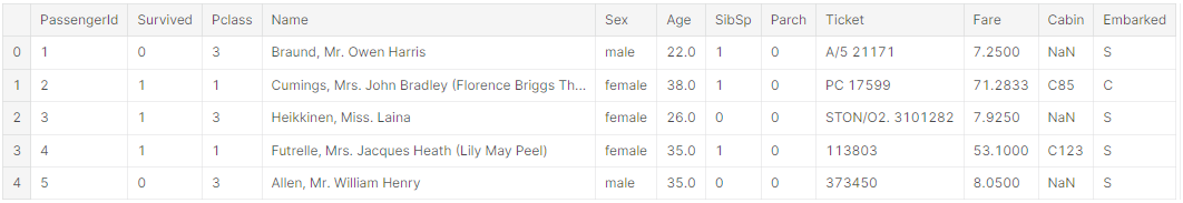
데이터 유형이 섞인 feature는 무엇인가?
- 같은 feature 안에 수치형과 영숫자형이 있을 수 있다. correcting 목적에 이런 feature가 포함된다.
- Ticket = 수치 + 영숫자
- Cabin = 영숫자형
오타나 오류를 포함하고 있는 feature는 무엇인가
- 큰 데이터셋을 다 살펴보기에는 힘들지만, 적은 데이터셋에서 몇 개의 샘플들을 살펴봤을 때 보이는 오류 혹은 오타는 correcting이 필요하다고 볼 수 있다.
- Name는 오류 혹은 오타를 포함하고 있을 수 있다. 줄인 이름이거나 별명을 쓰기 위해 괄호나 인용 기호
train_df.tail()
빈칸이나 null 혹은 빈 값을 가지고 있는 feature는 무엇인가
- 이런 feature들은 correcting이 필요하다.
- Cabin > Age > Embarked features는 training dataset에 null 값을 포함하고 있다.
- Cabin > Age 는 test 데이터셋에서 불완전하다.
features의 데이터 타입은 무엇인가?
- 데이터 타입을 아는 것은 converting을 하는 과정에서 도움이 된다.
- 7개의 features는 integer 나 float이다. test dataset에는 6개가 integer 혹은 float이다.
- 5개의 features는 string(object)이다.
train_df.info()
print('_'*40)
test_df.info()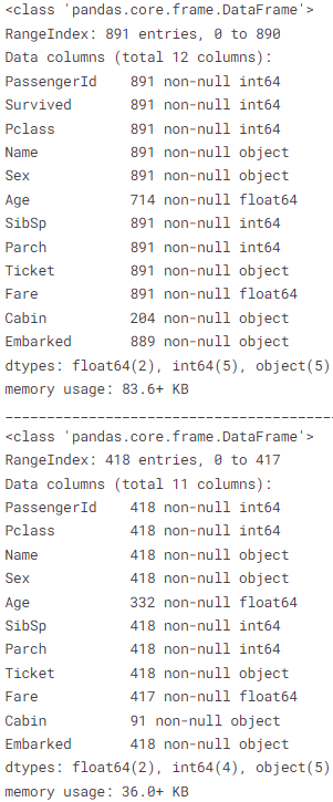
samples 중에서 숫자 features의 distribution은?
- feature의 distribution은 다른 초기의 insights, 실제 문제 도메인의 training dataset이 얼마나 대표적인가 중에서 결정하는 것을 돕는다.
- 전체 샘플들은 891, 실제 타이타닉호에 탑승한 승객(2,224)의 40% 이다.
- 'Survived'인 범주형 feature는 0 혹은 1의 값을 가진다.
- 약 38% samples이 실제 생존율의 32%의 생존 대표성을 가진다.
- 대부분의 승객 (>75%) 부모 혹은 아이와 여행하지 않았다.
- 승객의 30%가 형제나 배우자가 있었다.
- 요금은 $512를 내는 정도를 내는 승객(<1%)이 거의 없을 정도로 다양했다.
- 65~80세의 노인 승객(<1%)은 거의 없었다.
train_df.describe()
# Review survived rate using 'percentiles=[.61, .62]' knowing our problem description mentions 38% survival rate.
# Review Parch distribution using 'percentile=[.75, .8]'
# SibSp distribution '[.68, .69]'
# Age and Fare '[.1, .2, .3, .4, .5, .6, .7, .8, .9, .99']'
범주형 features의 distribution은?
- dataset에서 Names은 중복되지 않는다. (count = unique = 891)
- Sex 변수는 두 가지 값이 가능하다. male=65% (top = male, freq = 577 / count = 891)
- Cabin 변수는 몇 가지의 중복되는 샘플들이 있다. 혹은 몇 명의 승객들이 방을 공유했다는 것을 의미한다.
- Embarked는 3가지의 값이 가능하다. 대부분의 승객들은 S 포트를 사용한다. (top = S)
- Ticket은 가장 높은 비율(22%)로 중복값이 많다. (unique = 681)
train_df.describe(include=['O'])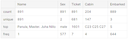
데이터 분석을 통한 추측
다음에 적절한 단계를 하기 위해서 데이터 분석을 통해 더 나은 추측을 하려고 한다.
- Correlating
- 각각의 feature가 생존과 얼마나 상관관계가 있는가를 알아야 한다. 프로젝트 초기에 상관관계 계산하고 후반에 상관관계를 빠르게 매치시켜야 한다.
- Completing
- 'Age'와 생존과의 완벽한 상관관계가 있는지를 확실히 해야 한다.
- 'Embarked'가 생존과 상관관계가 있는지 혹은 다른 중요한 feature와 상관관계가 있는지 확실히 해야 한다.
- Correcting
- 'Ticket'은 위의 분석에 따르면 삭제해야 한다. 가장 높은 중복 데이터(22%)를 가지고 있고 생존과 상관관례를 찾을 수 없다.
- 'Cabin'은 높은 불완전성을 가지며 training 데이터셋, test 데이터셋 모두에서 null 값을 많이 가지고 있기 때문에 삭제.
- 'PassengerId'는 생존에 아무런 연관이 없기 때문에 training 데이터셋에서 삭제되어야 한다.
- 'Name'은 상대적으로 비표준적이며, 생존과 직접적인 연관이 없다. 따라서 삭제되어야 한다.
- Creating
- 'Parch'와 'SibSp'를 기반으로 'Family'라는 새로운 feature를 생성. 승객 중에서 전체 가족의 수가 얼마나 되는지 알기 위해서.
- 'Name'을 가지고 'Title'이라는 새로운 feature를 추출할 것.
- 'Age band(연령층)'이라는 새로운 feature 생성. 연속적 숫자 feature에서 ordinal categorical feature로 바뀔 것.
- 'Fare range(요금 범위)'이라는 feature 생성.
- Classifying
- 앞서 문제에 대해 작성한 여러 설명을 기반으로 추측(가설)을 추가
- 여성 (Sex = female)은 생존율이 높다.
- 어린이 (Age < ?)는 생존율이 높다.
- 더 좋은 자리를 가진 승객 (Pclass = 1)은 생존율이 높다.
Analyze by pivoting features
pivoting이란?
1차 연립 방정식에서의 주축 방정식을 가려내는 기법을 통틀어서 피버팅이라 하며, 행렬에서 소거법을 수행할 때, 행 연산 규칙을 적용하여 계수 행렬 원소 가운데 절댓값이 가장 큰 원소가 대각선상에 오도록 해서 이 원소를 피벗 원소로 택하는 방법.
Data pivoting?
다른 관점에서 데이터를 볼수 있도록 열과 행을 재정렬하는 것.
관찰한 것들과 추측을 확인하기 위해서, 각각의 features를 pivoting하면서 빨리 분석할 수 있다. features에 빈 값이 없는 단계에서만 가능하다. 범주형(Sex), Ordinal(Pclass), 이산형(SibSp, Parch) features일 때만 말이 된다.
- Pclass
- 생존과 Pclass=1 사이(Classifying #3)의 엄청난 상관관계(>0.5)를 볼 수 있다. 따라서 모델이 이 feature를 포함할 것. - Sex
- Sex = female 일 때 높은 생존율(74%)을 보인다.(classifying #1) 따라서 문제를 해결한다고 볼 수 있다. - SibSp and Parch
- 이 features는 어떤 특정한 값과 상관 관계가 없다. 그래서 각각의 feature에서 새로이 만들어지거나 합쳐진 feature가 좋을 것이다. (creating #1)
<아래의 코드들은 생존이라는 feature와 각각의 feature의 상관관계를 파악하기 위함>
train_df[['Pclass', 'Survived']].groupby(['Pclass'], as_index=False).mean().sort_values(by='Survived', ascending=False)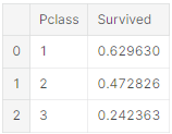
train_df[['Sex', 'Survived']].groupby(['Sex'], as_index=False).mean().sort_values(by='Survived', ascending=False)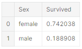
train_df[['SibSp', 'Survived']].groupby(['SibSp'], as_index=False).mean().sort_values(by='Survived', ascending=False)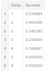
train_df[['Parch', 'Survived']].groupby(['Parch'], as_index=False).mean().sort_values(by='Survived', ascending=False)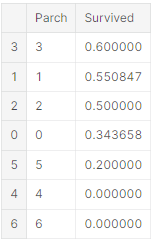
Analyze by visualizing data
데이터를 시각화하여 분석하면서 어떤 feature를 사용하는 것이 좋을지 확실히 할 것.
숫자 feature의 상관관계성
생존이라는 목표와 숫자 feature 사이의 상관관계를 이해하려고 한다.
히스토그램 차트는 나이와 같은 계속적인 숫자 변수를 분석하는 데에 좋다. 히스토그램은 자동으로 갯수나 같은 범위를 사용하여 샘플들의 분포를 나타낸다. 이 그래프는 우리가 질문과 관련된 특정 영역을 통해 답을 찾을 수 있도록 도와준다. (유아(4-7세)의 생존율이 더 높은가?)
히스토그램의 x축은 샘플들(승객들)의 수를 나타낸다.
- Observations
- 유아 (Age <= 4) 는 높은 생존율을 갖는다.
- 최고령자인 승객 (Age = 80)은 살았다.
- 가장 많은 수의 승객인 15-25세는 살아남지 못했다.
- 대부분의 승객들은 13-35세 사이이다.
- Decisions
간단한 분석을 한 후 다음 단계로 넘어갈 것.
- 모델 학습을 할 때는 'Age'(classifying #2)를 무조건 포함해야 함.
- 'Age'에서 null 값이 있지 않도록 완성한다. (completing #1)
- 나이를 일정한 그룹으로 나눠야 한다. (creating #3)
g = sns.FacetGrid(train_df, col='Survived')
g.map(plt.hist, 'Age', bins=20)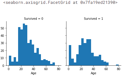
숫자와 ordinal features의 상관관계성
하나의 그래프로 상관관계를 파악하기 위해서 여러 개의 features를 합칠 수 있다. 숫자 값을 갖는 범주형 feature와 숫자 feature로 할 수 있다.
- Observations
- 대부분의 승객들은 Pclass = 3 이지만, 살아남지 못했다. classifying #2
- Pclass = 2 와 Pclass = 3인 유아 승객은 거의 살았다. 더 나은 결과를 얻기 위해서 classifying #2
- Pclass = 1의 대부분의 승객들은 살았다. classifying #3
- Pclass는 승객들의 나이 분포에 따라서 다르다.
- Decisions
- 모델 학습에 Pclass를 포함한다.
# grid = sns.FacetGrid(train_df, col='Pclass', hue='Survived')
grid = sns.FacetGrid(train_df, col='Survived', row='Pclass', size=2.2, aspect=1.6)
grid.map(plt.hist, 'Age', alpha=.5, bins=20)
grid.add_legend();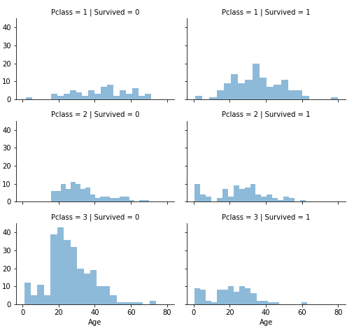
범주형 features 상관관계성
- Observations
- 여성 승객이 남성 승객보다 생존율이 높다 (classifying #1)
- Embarked=C 인 경우를 제외하고 여성들이 높은 생존율을 가진다. 이는 Pclass와 Embarked의 상관관계가 Pclass와 Survived의 상관관계가 될 수도 있음을 볼 수 있지만, 꼭 Embarked와 Survived의 직접적인 상관관계가 있다고는 할 수 없다.
- C와 Q 포트에서 Pclass=2인 경우와 비교했을 때, Pclass=3인 남성의 생존률이 더 높다. (Completing #2)
- Pclass=3이면서 남성 승객인 경우 출항지는 다양한 생존률을 가진다. - Decisions
- 모델 학습에 성별('Sex')을 추가
- 'Embarked'를 완성시켜서 모델 학습에 추가
# grid = sns.FacetGrid(train_df, col='Embarked')
grid = sns.FacetGrid(train_df, row='Embarked', size=2.2, aspect=1.6)
grid.map(sns.pointplot, 'Pclass', 'Survived', 'Sex', palette='deep')
grid.add_legend()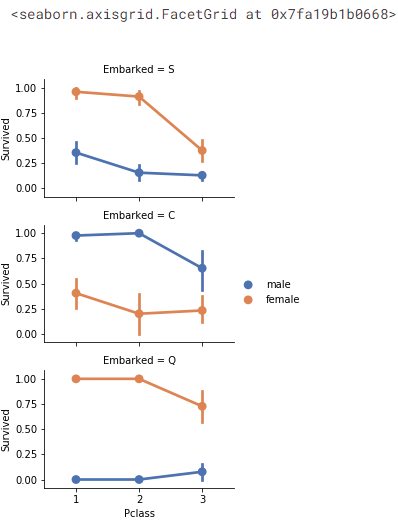
범주형과 숫자 features의 상관관계성
Embarked(Categorical non-numeric), Sex(Categorical non-numeric), Fare(Numeric continuous), with Survived(Categorical numeric)
- Observations
- 높은 요금을 낸 승객일수록 생존 가능성이 높다. (creating #4 요금 범위)
- 출항지와 생존률의 상관관계 (correlating #1 and completing #2)
- Decisions
- 요금 범위를 고려할 것.
# grid = sns.FacetGrid(train_df, col='Embarked', hue='Survived', palette={0: 'k', 1: 'w'})
grid = sns.FacetGrid(train_df, row='Embarked', col='Survived', size=2.2, aspect=1.6)
grid.map(sns.barplot, 'Sex', 'Fare', alpha=.5, ci=None)
grid.add_legend()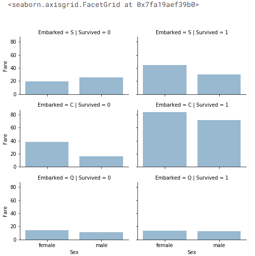
Wrangle data
원하는 결과를 얻기 위해서 위에서 모델 학습을 위해서 결정한 여러가지 중에서 몇 개만 정할 것.
위의 결과에 따라서 correcting, creating, completing을 할 것.
Correcting by dropping features
목표를 실행하기에 가장 좋은 시작~ features를 삭제하면 적은 features로 데이터를 다뤄야 한다. 분석이 쉬워지고 모델 실행이 빨라진다.
위의 assumptions와 decisions로 Cabin(correcting #2)과 Ticket(correcting #1)을 삭제한다.
일관성을 유지하기 위해서 training set과 test set 모두에 적용되는 것임을 명심!
print("Before", train_df.shape, test_df.shape, combine[0].shape, combine[1].shape)

train_df = train_df.drop(['Ticket', 'Cabin'], axis=1)
test_df = test_df.drop(['Ticket', 'Cabin'], axis=1)
combine = [train_df, test_df]

print("After", train_df.shape, test_df.shape, combine[0].shape, combine[1].shape)
Creating new feature extracting from existing
'Name'과 'PassengerId'를 삭제하기 전에, 'Name'에서 title을 뽑아내고 title과 'survival' 사이의 상관관계를 테스트하기 위해 'Name'을 가공할 수 있는지 확인하고 싶음.
정규식을 사용하여서 'Name'에서 'Title'을 따고 싶다. RegEx 패턴 (\w+\.) 'Name'에서 첫 단어가 점(.)으로 끝나는 단어를 뜻한다. expand=False 은 DataFrame을 반환한다.
-
Observations
Title, Age, ans Survived
- 대부분의 Age 범위 그룹은 정확하다. ex)
- Title과 Age 범위 사이의 생존은 다양하다.
- 특정 titles(Mme, Lady, Sir)은 대부분 살지만, 아니면(Don, Rev, Jonkheer) 살지 못한다. -
Decisions
- 모델 학습에 'Title'을 유지하기로 함
for dataset in combine:
	dataset['Title'] = dataset.Name.str.extract('([A-Za-z]+)\.', expand=False)

pd.crosstab(train_df['Title'], train_df['Sex'])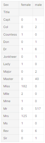
titles를 흔한 이름으로 치환하거나 Rare로 분류할 수 있다.
for dataset in combine:
	dataset['Title'] = dataset['Title'].replace(['Lady', 'Countess', 'Capt', 'Col', 'Don', 'Dr', 'Major', Rev', 'Sir', 'Jonkheer', 'Dona'], 'Rare')

    dataset['Title'] = dataset['Title'].replace('Mlle', 'Miss')
    dataset['Title'] = dataset['Title'].replace('Ms', 'Miss')
    dataset['Title'] = dataset['Title'].replace('Mme', 'Mrs')

train_df[['Title', 'Survived']].groupby(['Title'], as_index=False).mean()
범주형 titles을 ordinal로 바꿀 수 있다.
title_mapping = {'Mr': 1, 'Miss': 2, 'Mrs': 3, 'Master': 4, 'Rare': 5}

for dataset in combine:
	dataset['Title'] = dataset['Title'].map(title_mapping)
    dataset['Title'] = dataset['Title'].fillna(0)

train_df.head()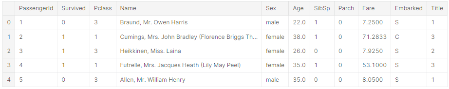
training, testing datasets에서 'Name'을 안전하게 삭제할 수 있다. training dataset에 있는 PassengerId도 필요없다.
train_df = train_df.drop(['Name', 'PassengerId'], axis=1)
test_df = test_df.drop(['Name'], axis=1)
combine = [train_df, test_df]
train_df.shape, test_df.shape
범주형 features 바꾸기
문자열을 가지고 있는 features를 숫자로 바꿀 수 있다. 모델 알고리즘에 적용하기 위해서 필요하나 작업이다. feature를 완성시키는 목표에 다다를 수 있게 돕는다.
'Sex'를 female=1, male=0인 'Gender'라는 새로운 feature로 바꾼다.
for dataset in combine:
	dataset['Sex'] = datset['Sex'].ma[({'female': 1, 'male': 0}).astype(int)

train_df.head()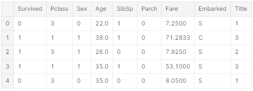
연속적 숫자 feature 완성하기
결측값이나 널값을 측정하고 완성시켜야 한다. Age를 먼저 시작.
연속적 숫자 feature를 다루는 3가지 방법이 있음.
- 평균과 표준 편차 사이의 랜덤 값을 생성하는 간단한 방법
- 결측값을 추정하는 더 정확한 방법은 다른 상관관계의 features를 사용하는 것이다.
Age, Gender, Pclass 사이의 상관관계를 주목해보자.
Pclass와 Gender가 합쳐진 sets에서 Age의 평균값을 사용하여 Age의 값을 추정할 수 있다.
그러니까, Pclass=1, Gender=0에서 평균 나이, Pclass=1, Gender=1에서의 평균 나이 이렇게 할 수 있다. - 방법 1과 2를 합치는 방법. 평균값으로 나이값을 추정하는 대신 Pclass와 Gender가 합펴진 sets에서 평균값과 표준 편차 사이의 랜덤값을 사용하는 것이다.
방법 1, 3은 우리 모델에 노이즈가 발생(여러 번 실행했는데 결과가 달랐다)하기 때문에 2번을 사용할 것.
# grid = sns.FacetGrid(train_df, col='Pclass', hue='Gender')
grid = sns.FacetGrid(train_df, row='Pclass', col='Sex', size=2.2, aspect=1.6)
grid.map(plt.hist, 'Age', alpha=.5, bins=20)
grid.add_legend()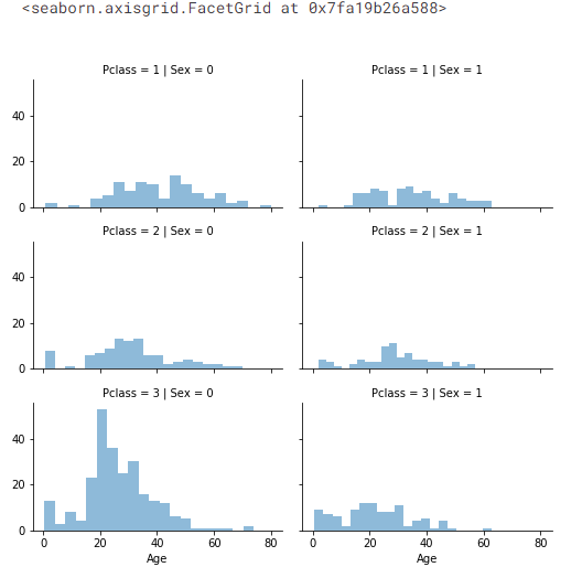
먼저, Pclass x Gender를 기반으로 추측한 나이값을 포함하기 위한 빈 배열을 생성
guess_ages = np.zeros((2,3))
guess_ages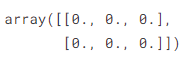
Sex(0 or 1) 과 Pclas(1,2,3)을 반복하면서 여섯 가지의 추측할 수 있는 나이값을 계산
for dataset in combine:
	for i in range(0,2):
    	for j in range(0,3):
        	guess_df = dataset[(dataset['Sex'] == i) & (dataset['Pclass'] == j+1)['Age'].dropna()

            # age_mean = guess_df.mean()
            # age_std = guess_df.std()
            # age_guess = rnd.uniform(age_mean - age_std, age_mean + age_std)

            age_guess = guess_df.median()

            # Convert random age float to nearest .5 age
            guess_ages[i,j] = int(age_guess / 0.5 + 0.5) * 0.5

	for i in range(0,2):
    	for j in range(0,3):
        	dataset.loc[(dataset.Age.isnull()) & (dataset.Sex == i) & (dataset.Pclass == j+1), 'Age'] = guess_ages[i,j]

	dataset['Age'] = datset['Age'].astype(int)

train_df.head()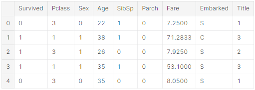
나이 범위를 설정하고 생존과의 상관관계를 살펴볼 것
train_df['AgeBand'] = pd.cut(train_df['Age'], 5)
train_df[['AgeBand', 'Survived']].groupby(['AgeBand'], as_index=False).mean().sort_values(by='AgeBand', ascending=True)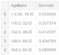
원래 나이값을 나이 범위로 바꿈
for dataset in combine:
	dataset.loc[dataset['Age'] <= 16, 'Age'] = 0
    dataset.loc[(dataset['Age'] > 16) & (dataset['Age'] <= 32), 'Age'] = 1
    dataset.loc[(dataset['Age'] > 12> & (dataset['Age'] <= 48), 'Age'] = 2
    dataset.loc[(datset['Age'] > 48) & (dataset['Age'] <= 64), 'Age'] = 3
    dataset.loc[dataset['Age'] > 64, 'Age']
train_df.head()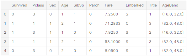
'AgeBand'를 삭제할 수 없음
train_df = train_df.drop(['AgeBand'], axis=1)
combine = [train_df, test_df]
train_df.head()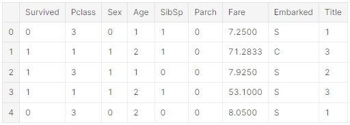
있는 features의 조합으로 새로운 feature 만들기
Parch와 SibSp를 합쳐서 FamilySize라는 새로운 feature를 생성할 수 있다. 그리고 Parch와 SibSp를 삭제할 것.
for dataset in combine:
	dataset['FamilySize'] = dataset['SibSp'] + datset['Parch'] + 1

train_df[['FamilySize', 'Survived']].groupby(['FamilySize'], as_index=Flase).mean().sort_values(by='Survived', ascending=False)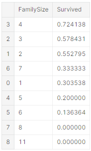
IsAlone이라는 feature를 생성
for dataset in combine:
	dataset['IsAlone'] = 0
    dataset.loc[dataset['FamilySize'] == 1, 'IsAlone']

train_df[['IsAlone', 'Survived']].groupby(['IsAlone'], as_index=False).mean()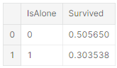
IsAlone을 사용하고 Parch, SibSp, FamilySize는 삭제
train_df = train_df.drop(['Parch', 'SibSp', 'FamilySize'], axis=1)
test_df = test_df.drop(['Parch', 'SibSp', 'FamilySize'], axis=1)
combine = [train_df, test_df]

train_df.head()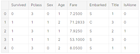
artificial feature = Pclas * Age
for dataset in combine:
	dataset['Age*Class'] = dataset.Age * dataset.Pclass

train_df.loc[:,['Age*Class', 'Age', 'Pclass']].head(10)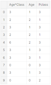
범주형 feature 완성시키기
항만에 따라서 Embarked은 S, Q, C를 가질 수 있다. training dataset은 두 개의 결측값이 있다. 그래서 결측값을 빈도가 높은 값으로 채울 것이다.
freq_port = train_df.Embarked.dropna().mode()[0]
freq_port
'S'
for dataset in combine:
	dataest['Embarked'] = dataset['Embarked'].fillna(freq_port)
train_df[['Embakred', 'Survived']].groupby(['Embarked'], as_index=False).mean().sort_values(by='Survived', ascending=False)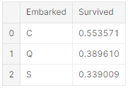
범주형 feature를 숫자로 바꾸기
새로운 숫자 Portfeature를 생성해서 EmbarkedFill를 바꿀 수 있다.
for dataset in combine:
	dataset['Embarked'] = dataset['Embarked'].map({'S': 0, 'C': 1, 'Q': 2}).astype(int)

train_df.head()
숫자 feature를 완성시키고 바꾸기
Fare에 가장 많이 나타나는 값을 찾아서 그 값을 test dataset의 결측값에 채워넣을 수 있다. 코드 한 줄로 가능
새로운 feature를 중간에 생성하거나 결측값을 채울 때 추가 상관관계 분석을 하지 않음을 주의!!
완성 목표는 널값이 없는 데이터에서 동작하는 모델 알고리즘에 주어진 요구사항을 달성하는 것이다.
요금 값을 소수점 두 자리까지 반올림 할 수 있다. (통용 가능)
test_df['Fare'].fillna(test_df['Fare'].dropna().median(), inplace=True)
test_df.head()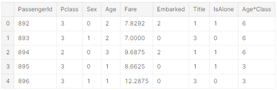
요금 범위는 생성할 수 없다.
train_df['FareBand'] = pd.qcut(train_df['Fare'], 4)
train_df[['FareBand', 'Survived']].groupby(['FareBand'], as_index=False).mean().sort_values(by='FareBand', ascending=True)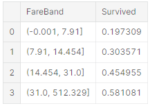
FareBand를 기반으로 Fare를 ordinal 값으로 바꿀 것.
for dataset in combine:
    dataset.loc[ dataset['Fare'] <= 7.91, 'Fare'] = 0
    dataset.loc[(dataset['Fare'] > 7.91) & (dataset['Fare'] <= 14.454), 'Fare'] = 1
    dataset.loc[(dataset['Fare'] > 14.454) & (dataset['Fare'] <= 31), 'Fare']   = 2
    dataset.loc[ dataset['Fare'] > 31, 'Fare'] = 3
    dataset['Fare'] = dataset['Fare'].astype(int)

train_df = train_df.drop(['FareBand'], axis=1)
combine = [train_df, test_df]

train_df.head(10)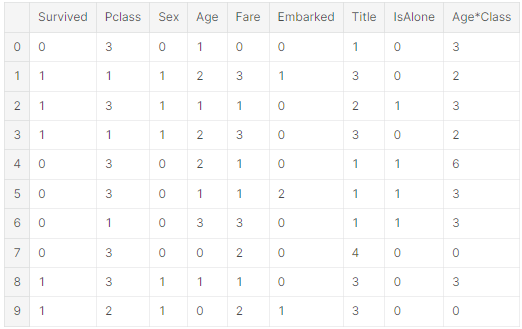
test_df.head(10)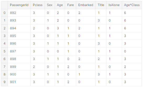
Model, predict and solve
모델을 학습시키고 예측할 준비가 됐다. 60개 이상의 예측 모델링 알고리즘이 있다. 문제 유형과 해결 조건을 파악하여 평가할 수 있는 몇 개의 모델들을 좁혀가며 선택하면 된다. 우리 문제는 분류와 회귀 문제다. features(Gender, Age, Port ...)혹은 어떠한 값들과 출력(생존인가 아닌가)의 사이의 관계를 파악해야 한다. 주어진 데이터셋으로 모델을 학습시키는 지도학습의 머신러닝을 실행할 것이다. 이렇게 두 가지의 기준(지도학습 + 분류, 회귀)으로 여러가지의 모델들 중에서 몇 가지로 추릴 수 있다.
<예측 모델링 알고리즘>
- Logistic Regression
- KNN or k-Nearest Neighbors
- Support Vector Machines
- Naive Bayes classifier
- Decision Tree
- Random Forest
- Preceptron
- Artificial neural network
- RVM or Relevance Vector Machine
X_train = train_df.drop('Survived', axis=1)
Y_train = train_df['Survived']
X_test = test_df.drop('PassengerId', axis=1).copy()
X_train.shape, Y_train.shape, X_test.shape
Logistic Regression
Logistic Regression은 workflow의 초기에 실행할 수 있는 유용한 모델이다. Logistic regression은 누적 로지스틱 분포인 로지스틱 함수를 사용해서 확률을 추정해서 범주형 속 변수(feature)와 하나 이상의 독립 변수(features)의 관계를 측정한다.
training dataset을 기반으로 한 모델에서 confidence score가 생성됨을 주의!!
# Logistic Regression
logreg = LogisticRegression()
logreg.fit(X_train, Y_train)
Y_pred = logreg.predict(X_test)
acc_log = round(logreg.score(X_train, Y_train) * 100, 2)
acc_log
80.3.6
Logistic Regression은 completing goals과 feature creating을 위한 decisions과 assumptions을 입증하기 위해 사용할 수도 있다. decision function의 features의 계수를 계산해서 입증할 수 있다.
계수가 양수이면 log-odds 가 증가(확률이 증가)하고 계수가 음수이면 log-odds가 감소(확률이 감소)한다.
Sex는 가장 큰 양수 계수이며, 값이 증가하면 Survived=1일 확률이 증가한다.- 반대로 Pclass가 증가하면 Survived=1일 확률이 감소한다.
- 그래서 Age*Class는 좋은 artificial feature다. Survived와 두 번째로 큰 음의 상관관계를 갖기 때문.
- 그리고 Title이 두 번째로 큰 양의 상관관계를 갖는다.
coeff_df = pd.DataFrame(train_df.columns.delete(0))
coeff_df.columns = ['Featrue']
coeff_df['Correlation'] = pd.Series(logreg.coef_[0])

coef_df.sort_values(by='Correlation', ascending=False)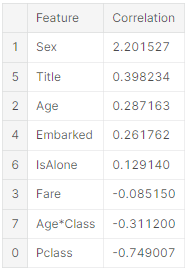
Support Vecotr Machines (SVM)
다음 모델은 Support Vecotr Machines을 사용해서 모델링할 것.
# Support Vector Machines

svc = SVC()
svc.fit(X_train, Y_train)
Y_pred = svc.predict(X_test)
acc_svc = round(svc.score(X_train, Y_train) * 100, 2)
acc_svc
83.84
KNN
knn = KNeighborsClassifier(n_neighbors = 3)
knn.fit(X_train, Y_train)
Y_pred = knn.predict(X_test)
acc_knn = round(knn.score(X_train, Y_train) * 100, 2)
acc_knn
84.74
Naive Bayes classifier
# Gaussian Naive Bayes

gaussian = GaussianNB()
gaussian.fit(X_train, Y_train)
Y_pred = gaussian.predict(X_test)
acc_gaussian = round(gaussian.score(X_train, Y_train) * 100, 2)
acc_gaussian
72.28
Perceptron
# Perceptron

perceptron = Perceptron()
perceptron.fit(X_train, Y_train)
Y_pred = perceptron.predict(X_test)
acc_perceptron = round(perceptron.score(X_train, Y_train) * 100, 2)
acc_perceptron
78.0
# Linear SVC

linear_svc = LinearSVC()
linear_svc.fit(X_train, Y_train)
Y_pred = linear_svc.predict(X_test)
acc_linear_svc = round(linear_svc.score(X_train, Y_train) * 100, 2)
acc_linear_svc
79.12
# Stochastic Gradient Descent

sgd = SGDClassifier()
sgd.fit(X_train, Y_train)
Y_pred = sgd.predict(X_test)
acc_sgd = round(sgd.score(X_train, Y_train) * 100, 2)
acc_sgd
78.56
Decision Tree
# Decision Tree

decision_tree = DecisionTreeClassifier()
decision_tree.fit(X_train, Y_train)
Y_pred = decision_tree.predict(X_test)
acc_decision_tree = round(decision_tree.score(X_train, Y_train) * 100, 2)
acc_decision_tree
86.76
Random Forest
# Random Forest

random_forest = RandomForestClassifier(n_estimators=100)
random_forest.fit(X_train, Y_train)
Y_pred = random_forest.predict(X_test)
random_forest.score(X_train, Y_train)
acc_random_forest = round(random_forest.score(X_train, Y_train) * 100, 2)
acc_random_forest
86.76
Model evaluation
models = pd.DataFrame({
    'Model': ['Support Vector Machines', 'KNN', 'Logistic Regression',
              'Random Forest', 'Naive Bayes', 'Perceptron',
              'Stochastic Gradient Decent', 'Linear SVC',
              'Decision Tree'],
    'Score': [acc_svc, acc_knn, acc_log,
              acc_random_forest, acc_gaussian, acc_perceptron,
              acc_sgd, acc_linear_svc, acc_decision_tree]})
models.sort_values(by='Score', ascending=False)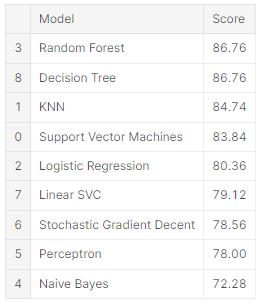
submission = pd.DataFrame({
        "PassengerId": test_df["PassengerId"],
        "Survived": Y_pred
    })
# submission.to_csv('../output/submission.csv', index=False)