https://arxiv.org/abs/1708.05031

요약

추천시스템 분야에서 기존에 쓰이던 MF에서 벗어나 DNN을 활용한 논문이다.

NCF 는 GMF와 MLP를 앙상블한 모델이다.
여기서 GMF는 MF에 non-linear activation function을 더해 표현력을 높인 MF이고,
MLP는 임베딩된 user Id와 itemID를 Input으로 받아 0~1의 $\hat y$를 구해주는 Multi-Layer-Perceptron이다.

Matrix Factorization의 문제점

참고 : Matrix Factorization 논문 리뷰 & 구현

MF는 두 벡터($p_u$:user u의 latent vector, $q_i$:item i의 latent vector)의 내적에 의해 $\hat y$ (predicted rating) 가 계산된다.
이 때 latent space는 서로 독립인 것을 가정하고 같은 가중치를 사용하여 선형결합을 통해 $\hat y$를 구하게 된다.

단순 선형 결합을 통해 $\hat y$을 구하기 때문에 user-item의 복잡한 상호작용을 온전히 표현할 수 없다.
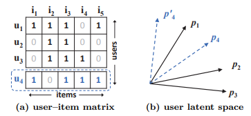
위 그림은 이런 MF의 표현력의 한계를 나타낸 그림이다.
만약 (a)에서 $u_4$와 유사한 순서를 $u_1$, $u_3$, $u_2$ 일 때, $u_4$를 $p_4$라는 latent vector로 보낸 것을 생각해 보자.

(b)를 보면 $u_4$와 유사도는 $u_3$가 $u_2$보다 높지만, $u_4$를 $p_4$ 라는 latent vector로 맵핑 시켰을 때 $p_2$에 더 유사하게 맵핑된 것을 볼 수 있다.(어떤 식으로 해도 유사도의 순서에 맞게 배치되지 않는다)

이러한 모순을 해결하기 위해 latent space에 축을 하나더 추가 할 수 있지만, overfitting 을 야기 할 수 있다.

따라서 이런 단점을 해결하기 위해 선형결합 대신 Deep Neural Networks를 사용한다.

Input

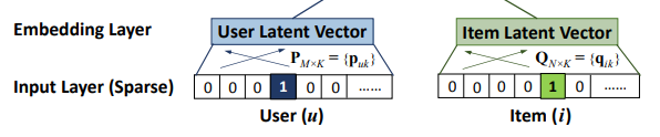
그림의 Input Layer에서 볼 수 있듯 유저와 아이템의 ID를 one-hot-encoding 하여 sparse한 vector로 변환하여 Input으로 사용한다.

예시)

각 User u 와 Item i 의 id를 one-hot-encoding
User u = [0,0,0,0,1,0,0,0]
Item i = [0,0,0,0,0,0,1,0,0,0,0]

그리고 Embedding Layer에서 Sparse한 one-hot-encoding 데이터를 Dense한 벡터로 바꿔준다.
이렇게 얻어진 dense vector은 Latent vector로도 볼 수 있다.

Model

모델에서 나오는 예측값 $\hat y_{u,i}$과 비교할 참값 $y_{u,i}$ 은 다음과 같다.

Implicit Feedback이기 때문에 1인 경우 interaction이 있었을 뿐 선호도를 반영하지 않고, 0인 경우 마찬가지로 item을 좋아하지 않는다는 것을 나타내지 않는다.

MLP

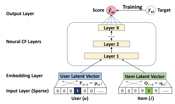
• Input data는 user, item을 각각 one-hot-encoding된 값이다. (Input Layer)
• Input을 Latent Vector로 각각 임베딩한다(Embedding Layer)
• 임베딩된 P (user Latent vector), Q (item Latent vector) 를 쌓여진 Layer에 올려 feed forward 한다 (Neural CF Layer)
• 최종 결과값($\hat y_{ui}$)는 0 ~ 1의 값을 가지게 출력한다. (Output Layer)
  - 그리고 $y_{ui}$와 비교하여 훈련을 진행 ( $y_{ui}$ = 0,1 )
  
  

위 과정을 수식으로 나타내면 다음과 같다.

GMF

MF가 NCF의 특별한 케이스가 됨을 보여준다.
앞서 Input에서 User와 Item 의 ID를 임베딩하여 Latent vector로 볼 수 있다.

첫번째 레이어를 맵핑하면 다음의 식과 같다.

$\phi_{1}\left(\mathbf{p}_{u}, \mathbf{q}_{i}\right)=\mathbf{p}_{u} \odot \mathbf{q}_{i}$

• ⊙는 성분곱
• $\mathbf{p}_{u} = \mathbf{P}^{T} \mathbf{v}_{u}^{U}$
• $\mathbf{q}_{i} = \mathbf{Q}^{T} \mathbf{v}_{i}^{I}$
  • 이때 P, Q 는 latent vector , v는 one-hot-encoding 된 vector

위 식을 output layer로 보내면 다음의 최종식이 나오게 된다.

$\hat{y}_{u i}=a_{o u t}\left(\mathbf{h}^{T}\left(\mathbf{p}_{u} \odot \mathbf{q}_{i}\right)\right)$

• $\mathbf{h}$ : activation function and edgeweights of the output layer
• $a_{o u t}$ : non-linear activation function(시그모이드 사용)

이렇게 만들어진 GMF식은 non-linear activation 을 추가하였기 때문에 기존의 MF보다 좋은 표현력을 가지게 된다.

※ $\mathbf{h}$ 와 $a_{o u t}$ 를 항등함수를 쓰면 기존의 MF가 된다.

GMF & MLP 혼합

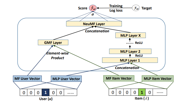
두 모델을 앙상블하는 간단한 솔루션은 GMF와 MLP가 동일한 Embedding Layer를 공유하게 하고, 그들의 인터랙션 기능들의 출력들을 결합하는 것이다. 그러나 GMF및 MLP의 Embedding을 공유하는 것은 융합된 모델의 성능을 제한할 수 있다.

이 논문에서는 융합된 모델에 flexibility를 주기 위해 GMF와 MLP를 서로 다른 embedding layer 사용하여
별도로 학습하고 마지막 은닉층을 concat하는 방법을 제안한다.

식으로 표현하면 다음과 같다.

• $\mathbf{p}_{u}^{G}$, $\mathbf{q}_{i}^{G}$ : GMF의 (user,item)latent vector
• $\mathbf{p}_{u}^{M}$, $\mathbf{q}_{i}^{M}$ : MLP의 (user,item)latent vector

Loss

likelihood function

Implicit feedback은 0,1로 이루어져 있기 때문에 $\hat y_{ui}$ 는 [0,1] 의 범위를 가지는 값을 출력하기 위해 Logistic 이나 Porbit을 사용하여 확률적 접근을 한다.

• $\mathcal Y$ : 관측된 집단 -> ${y}_{u i}$ = 1
• $\mathcal Y^-$ : 관측되지 않은 집단 ->${y}_{u i}$ = 0

Binaray cross-entropy loss

likelihood function 에 $-log$를 취하면 다음과 같은 Binaray cross-entropy loss식을 얻을 수 있다.

NCF에서는 이 Binaray cross-entropy loss를 가지고 Loss를 계산하게 된다.

Contribution

• 추천시스템에 Deep Neural Network 적용
• MF는 NCF의 특별한 케이스가 됨을 증명
• 여러 실험을 통한 NCF의 효율성 증명

논문 모르는 용어

Point-wise loss : 한번에 1개의 아이템만 고려

• 기존 Explicit Data에서 사용 ( True_rating - Predicted_ratin )

Pair-wise loss : 한번에 2개의 아이템을 고려

• (Positive item - 관측된 데이터, Negative item - 관측되지 않은 데이터)

Sparse Representation : 아이템 가지수 = 차원의 수 (원핫인코딩)

• ex) a = [1, 0, 0, 0, 0, 0, 0, 0, 0], b = [0, 1, 0, 0, 0, 0, 0, 0, 0] (0 or 1)

Dense Representation : 아이템 가지수 >> 차원의 수

• ex) a = [0.2,1.4,-0.4], b = [0.1, 0.5, 1.1] (실수값으로 이루어짐)