[LG헬로비전 DX DATA SCHOOL 4기] Python(9) (250116)

// 실습 코드
import seaborn as sns
import matplotlib.pyplot as plt

# 데이터셋 로드
tips = sns.load_dataset("tips")

# KDE Plot 생성
sns.kdeplot(
    tips['total_bill'],   # KDE 플롯에 사용할 데이터(총 계산 금액)
    fill=True    # 곡선 아래를 채워서 그래프를 시각적으로 강조    # 나중에 업데이트 되면 shade=True는 사용불가
)
plt.show()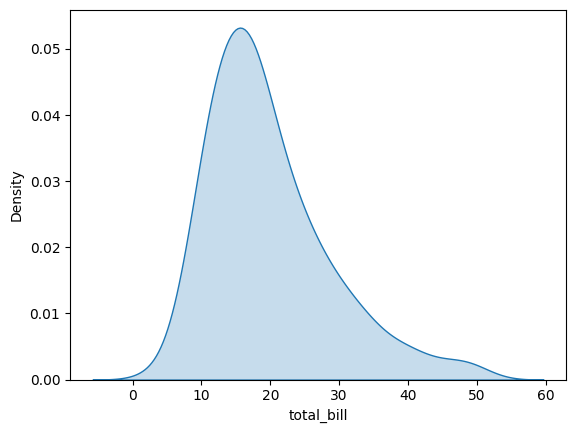

// 실습 코드
# rugplot : 데이터 분포의 각 데이터 포인트를 표시하는 간단한 그래프
tips = sns.load_dataset("tips")

sns.rugplot(
    data = tips,
    x = "total_bill",
    height = 0.5,
    color = 'blue'
)
plt.show()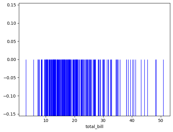

Heatmap
: heat + map / 데이터들의 배열을 색상으로 표현해주는 것.

=> 두 개의 카테고리 값에 대한 값 변화를 한눈에 알아보기 쉬움.

// 실습 코드
flights = sns.load_dataset('flights')   # 1949-1960년간 월별 승객 수를 담고 있는 데이터셋
print(flights)

// 실습 코드
df = flights.pivot(index='month', columns='year', values='passengers')
print(df)

ax = sns.heatmap(df)      # 빨간색에 짙을수록 승객수가 적음을 나타내고, 빨간색이 얕아질수록 승객수가 높음을 의미
plt.show()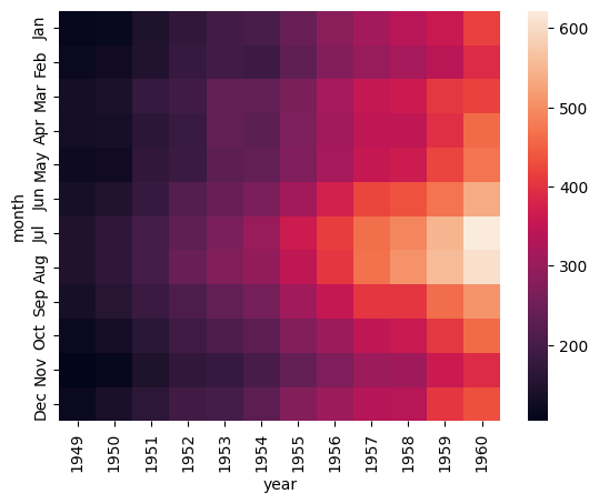

// 실습 코드
ax = sns.heatmap(df,  # 데이터
                 vmin = 100,  # 최솟값
                 vmax = 700,  # 최댓값
                 cbar = True, # colorbar의 유무
                 center = 400,  # 중앙값 선정
                 linewidths = 0.5,  # cell 사이에 선을 집어 넣는다.
                 annot = True,  # 숫자 표시
                 fmt = 'd', # 그 값의 데이터 타입 선정
                 cmap = 'Blues' # 히트맵의 색을 설정함
                 )
plt.show()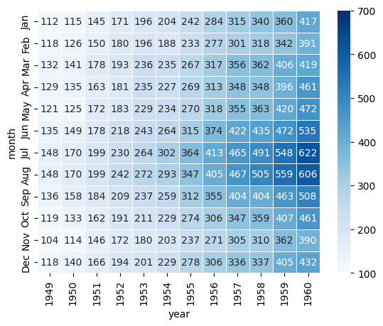

// 실습 코드
tips = sns.load_dataset('tips')
sns.lmplot(
    x = 'total_bill',
    y = 'tip',
    data = tips,
    hue = 'time',   # 색상을 시간(time : Lunch/Dinner)으로 구분
    markers = ['o', 'v'],
    height = 6,
    aspect = 1.5,
    scatter_kws = {'s':100, 'alpha':0.7}  # 점의 크기와 투명도 설정
)
plt.show()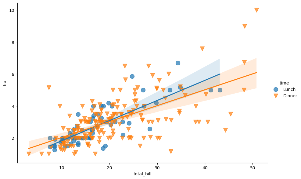

// 실습 코드
# pairplot    => 오래걸리는 단점
iris = sns.load_dataset('iris')

sns.pairplot(
    data = iris,
    hue = 'species',
    markers = ['o', 's', 'D']
)
plt.show()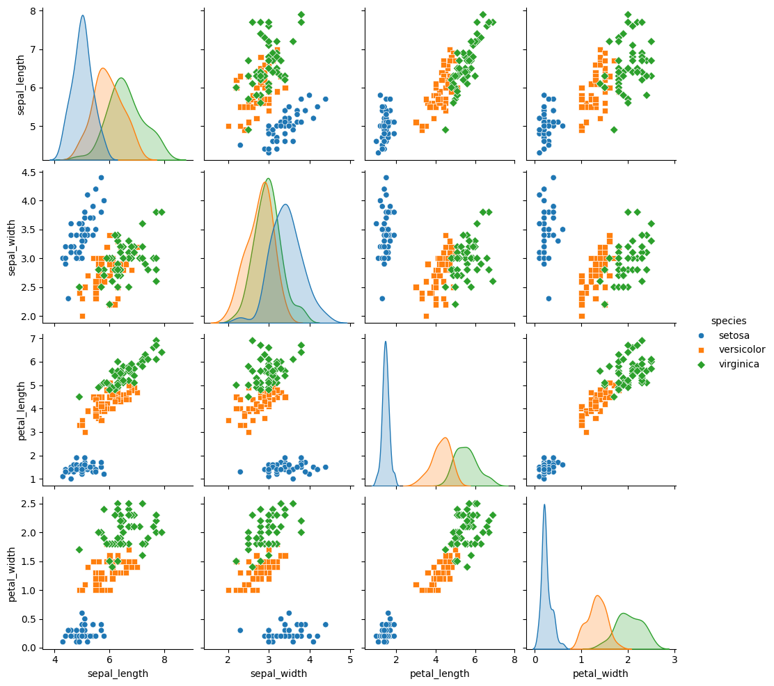

// 실습 코드
import seaborn as sns
import matplotlib.pyplot as plt
import pandas as pd

iris = sns.load_dataset("iris")

# 데이터 확인
print(iris.head())
print(iris.info())
print(iris.describe())

데이터 분포와 관계 심화(kdeplot)

// 실습 코드
features = ['sepal_length', 'sepal_width', 'petal_length', 'petal_width']
fig, axs = plt.subplots(2, 2, figsize=(12, 10)) # 2 x 2 구조

for i, feature in enumerate(features):
  row, col = divmod(i, 2) # 서브플롯의 행과 열 계산
  sns.kdeplot(
      data = iris,
      x=feature,
      hue='species',
      fill=True,
      alpha=0.6,
      ax = axs[row, col]
  )
  axs[row, col].set_title(f'Density plot of {feature}')

# 레이아웃 조정
plt.tight_layout()
plt.show()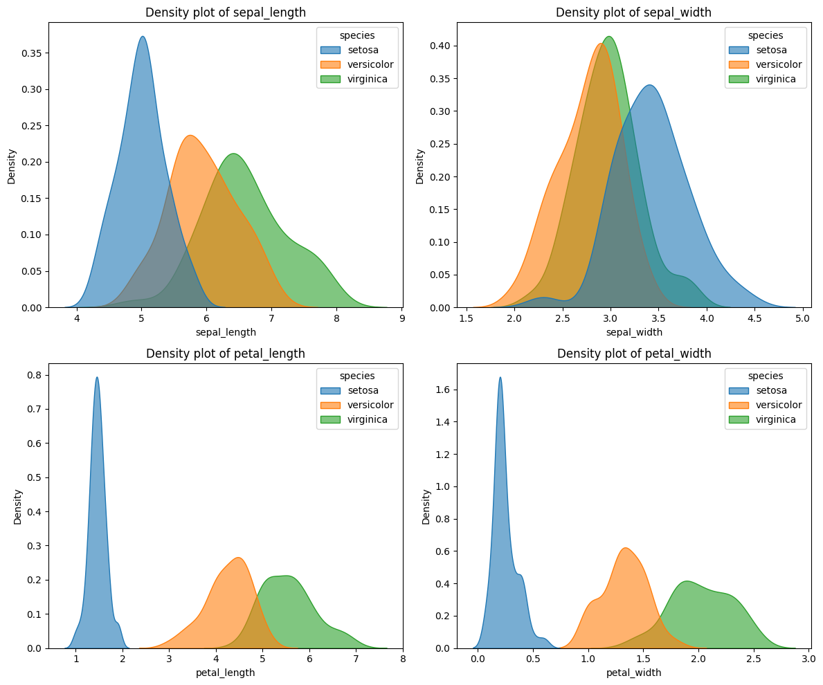

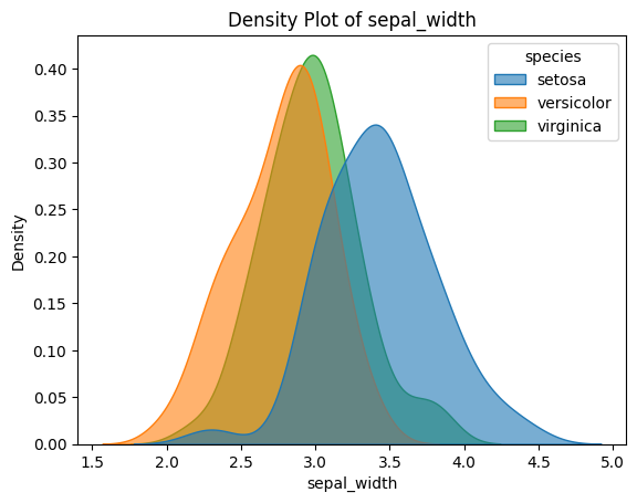
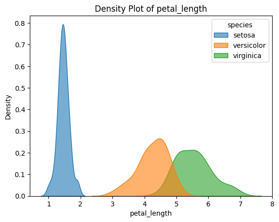
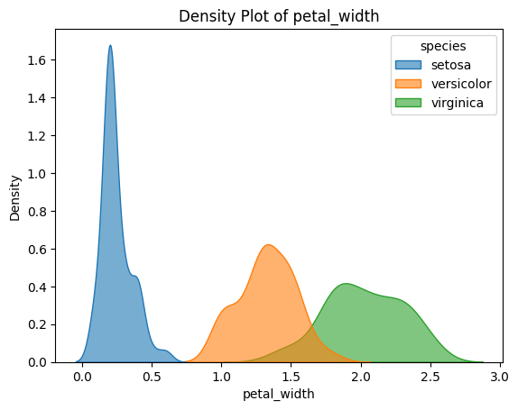
// 실습 코드
features = ['sepal_length', 'sepal_width', 'petal_length', 'petal_width']
for feature in features:
  sns.kdeplot(data = iris, x=feature, hue='species', fill=True, alpha=0.6)
  plt.title(f'Density Plot of {feature}')
  plt.show()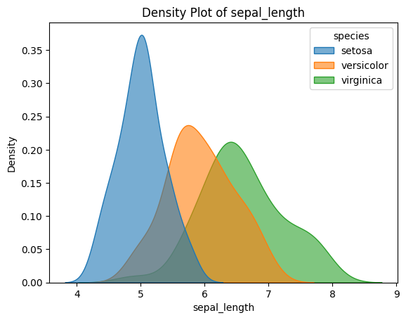

// 실습 코드
# swarmplot
sns.swarmplot(data = iris, x='species', y='sepal_length', palette='pastel')
plt.title("Sepal length Distribution by Species")
plt.show()

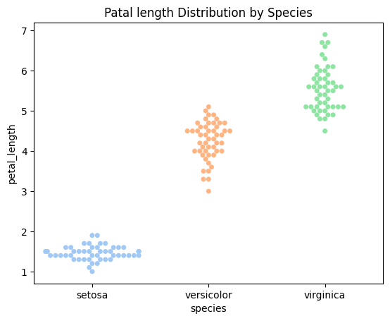
sns.swarmplot(data = iris, x='species', y='petal_length', palette='pastel')
plt.title("Patal length Distribution by Species")
plt.show()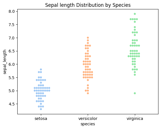

// 실습 코드
# Scatterplot + KDE 결합
sns.jointplot(data = iris, x='sepal_length', y='sepal_width', hue='species', kind='kde', fill=True)
plt.show

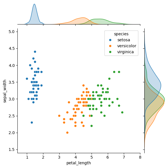
sns.jointplot(data = iris, x='petal_length', y='sepal_width', hue='species', kind='scatter')
plt.show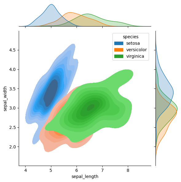

// 실습 코드
# Violinplot과 Stripplot 결합
sns.violinplot(data=iris, x='species', y='sepal_length', inner=None, palette='pastel')
sns.stripplot(data=iris, x='species', y='sepal_length', color='black', alpha=0.5)
plt.title('Violin + Strip plot : Sepal length by Sepcies')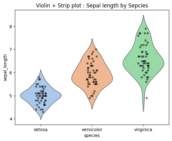

// 실습 코드
sns.pairplot(iris, hue='species', diag_kind='hist', palette='bright')
plt.show()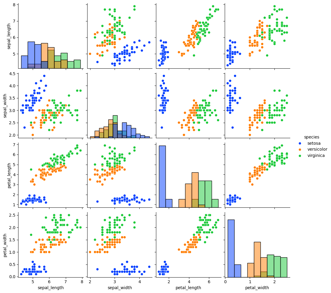

// 실습 코드
# 특성별 분포를 종별로 나눠 관찰
g = sns.FacetGrid(iris, col = 'species', height=4, aspect=1)
g.map(sns.histplot,'sepal_length', kde=True)
plt.show()

g = sns.FacetGrid(iris, col='species', height=4, aspect=1)
g.map(sns.histplot, 'petal_length', kde=True)
plt.show()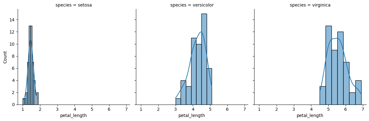

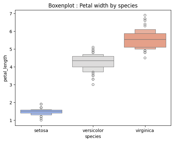
// 실습 코드
sns.boxenplot(data = iris, x='species', y='petal_length', palette='coolwarm')
plt.title('Boxenplot : Petal width by species')
plt.show()