분류

1. Classification(분류) 종류

Classification(분류): 다양한 머신러닝 알고리즘을 활용하여 데이터를 특정 클래스로 분류하는 작업

① 나이브 베이즈 (Naïve Bayes)

• 베이즈 정리를 기반으로 한 확률적 분류 알고리즘
• 독립 변수 간 독립성을 가정함
• 텍스트 분류(예: 스팸 필터링)에 자주 사용됨

② 로지스틱 회귀 (Logistic Regression)

• 선형 회귀를 기반으로 확률을 예측하는 기법
• 시그모이드(Sigmoid) 함수를 사용하여 출력 값을 0~1 사이로 변환
• 이진 분류(Binary Classification)에 자주 사용됨

③ 결정 트리 (Decision Tree)

• 데이터의 규칙을 기반으로 분류하는 알고리즘
• 트리 구조로 구성되며, 각 노드는 특정 특징을 기준으로 데이터를 분할
• 직관적이며 해석이 쉬우나 과적합(overfitting) 가능성이 있음

④ 서포트 벡터 머신 (Support Vector Machine, SVM)

• 클래스 간 최대 마진(Margin)을 찾는 방식으로 분류
• 초평면(Hyperplane)을 찾아 데이터를 분리
• 고차원 데이터에서도 성능이 우수하며, 커널 트릭(Kernel Trick)을 활용 가능

⑤ K-최근접 이웃 (K-Nearest Neighbor, KNN)

• 새로운 데이터가 들어오면 가장 가까운 K개의 이웃을 찾아 다수결로 분류
• 데이터가 많을수록 연산량이 커지는 단점이 있음
• 거리 기반으로 분류하므로 이상치(Outlier)에 민감함

⑥ 신경망 (Neural Network)

• 여러 개의 뉴런(Neuron)과 레이어(Layer)로 구성된 신경망 구조
• 비선형 문제 해결이 가능하며, 딥러닝(Deep Learning)에서 주로 사용됨
• 학습에 많은 데이터와 계산 자원이 필요함

⑦ 앙상블 (Ensemble)

• 여러 개의 머신러닝 모델을 조합하여 성능을 향상시키는 기법
• 대표적인 방법:
  • 배깅(Bagging, 예: 랜덤 포레스트)
  • 부스팅(Boosting, 예: XGBoost, AdaBoost)
• 단일 모델보다 일반적으로 성능이 우수함

---

2. 분류 성과 지표 (Classification Performance Metrics)

머신러닝 모델의 성능을 평가하기 위한 다양한 지표

① Confusion Matrix (혼동 행렬)

• 모델의 예측값과 실제값을 비교하여 정리한 표
• 구성 요소:
  • TP (True Positive): 실제 Positive이며, Positive로 예측한 경우
  • TN (True Negative): 실제 Negative이며, Negative로 예측한 경우
  • FP (False Positive): 실제 Negative인데 Positive로 예측한 경우 (Type I Error)
  • FN (False Negative): 실제 Positive인데 Negative로 예측한 경우 (Type II Error)

② Accuracy (정확도)

• 전체 데이터 중 올바르게 분류된 샘플의 비율
• (\text{Accuracy} = \frac{TP + TN}{TP + TN + FP + FN})
• 데이터가 불균형할 경우 정확도만으로 성능을 평가하는 것은 적절하지 않을 수 있음

③ Recall (재현율, Sensitivity)

• 실제 Positive 샘플 중에서 모델이 Positive로 예측한 비율
• (\text{Recall} = \frac{TP}{TP + FN})
• FN을 최소화하는 것이 중요한 문제(예: 질병 진단)에서 중요한 지표

④ Precision (정밀도)

• 모델이 Positive로 예측한 샘플 중 실제로 Positive인 비율
• (\text{Precision} = \frac{TP}{TP + FP})
• FP를 줄이는 것이 중요한 문제(예: 스팸 필터링)에서 중요한 지표

⑤ Specificity (특이도)

• 실제 Negative 샘플 중에서 모델이 Negative로 예측한 비율
• (\text{Specificity} = \frac{TN}{TN + FP})
• Recall과 반대되는 개념으로 활용됨

⑥ F1 Score

• 정밀도(Precision)와 재현율(Recall)의 조화 평균
• (\text{F1-score} = 2 \times \frac{\text{Precision} \times \text{Recall}}{\text{Precision} + \text{Recall}})
• 데이터 불균형 문제에서 유용함

⑦ ROC-AUC (Receiver Operating Characteristic - Area Under Curve)

• ROC 곡선은 모델의 모든 임계값(Threshold)에 대한 TPR(재현율)과 FPR(위양성률)을 나타냄
• AUC 값이 1에 가까울수록 좋은 성능을 의미함

오분류표(Confusion Matrix)

• 혼동 행렬(Confusion Matrix)은 분류 모델이 얼마나 정확하게 예측했는지를 평가하는 표
• 각 값들은 예측값과 실제값을 비교하여 분류 모델의 성능을 분석하는 데 사용됨

---

1. 혼동 행렬(Confusion Matrix)의 구조

	실제값 (Actual Values)
	Positive (암 O)
예측값 (Predicted Values)	Positive (암 O)
Negative (암 X)	FN (False Negative, Type II Error)

각 용어의 의미

• TP (True Positive): 실제 Positive 값(암 O)을 Positive(암 O)으로 올바르게 예측한 경우
• TN (True Negative): 실제 Negative 값(암 X)을 Negative(암 X)으로 올바르게 예측한 경우
• FP (False Positive, 1종 오류): 실제 Negative 값(암 X)인데 Positive(암 O)으로 잘못 예측한 경우
  → "없는데 있다고 판단한 오류"
  → 예: 건강한 사람을 암 환자로 오진함
• FN (False Negative, 2종 오류): 실제 Positive 값(암 O)인데 Negative(암 X)으로 잘못 예측한 경우
  → "있는데 없다고 판단한 오류"
  → 예: 암 환자를 건강하다고 오진함

---

2. 1종 오류(Type I Error) vs 2종 오류(Type II Error)

1종 오류 (False Positive, Type I Error)

• 귀무가설(H₀)이 참인데, 이를 기각하는 오류
• 실제로는 암이 없는데(음성), 암이 있다고 잘못 판단(양성)
  → "없는 것을 있다고 판단하는 오류"
  → 예: 건강한 사람을 암 환자로 오진 (잘못된 양성 진단)

2종 오류 (False Negative, Type II Error)

• 귀무가설(H₀)이 거짓인데, 이를 기각하지 않는 오류
• 실제로는 암이 있는데(양성), 암이 없다고 잘못 판단(음성)
  → "있는 것을 없다고 판단하는 오류"
  → 예: 암 환자를 정상이라고 오진 (잘못된 음성 진단)

의미

• 1종 오류를 줄이면: 암이 없는 사람을 환자로 잘못 진단하는 경우가 줄어듦
• 2종 오류를 줄이면: 실제 암 환자를 정상으로 오진하는 경우가 줄어듦 (더 위험한 상황)
• 일반적으로 2종 오류(FN)를 줄이는 것이 더 중요함 (ex: 질병 진단에서 암 환자를 놓치지 않는 것이 중요)

---

3. 혼동 행렬을 활용한 평가 지표

• 정확도(Accuracy): 전체 샘플 중에서 올바르게 예측한 비율
  [
  Accuracy = \frac{TP + TN}{TP + TN + FP + FN}
  ]
• 정밀도(Precision): 모델이 양성(Positive)이라고 예측한 샘플 중 실제로 양성인 비율
  [
  Precision = \frac{TP}{TP + FP}
  ]
• 재현율(Recall, Sensitivity): 실제 양성 샘플 중에서 모델이 양성으로 예측한 비율
  [
  Recall = \frac{TP}{TP + FN}
  ]
• 특이도(Specificity): 실제 음성(Negative) 샘플 중에서 모델이 음성으로 예측한 비율
  [
  Specificity = \frac{TN}{TN + FP}
  ]
• F1-Score: 정밀도와 재현율의 조화 평균
  [
  F1 = 2 \times \frac{Precision \times Recall}{Precision + Recall}
  ]
• ROC-AUC: 모델의 전체적인 성능을 평가하는 곡선(ROC)과 AUC 값

---

4. 오분류표(Confusion Matrix)의 활용

• 암 진단 모델에서 FN(2종 오류, False Negative)를 최소화하는 것이 중요 (암 환자를 정상으로 오진하면 치명적)
• 스팸 메일 필터링에서는 FP(1종 오류, False Positive)를 줄이는 것이 중요 (중요한 메일을 스팸으로 분류하면 불편함)
• 금융 사기 탐지에서는 정밀도(Precision)와 재현율(Recall)을 조절하여 적절한 균형을 맞춰야 함

---

K-Nearest Neighbors(KNN)

iris 꽃 종류 분류를 위한 시각화

// 실습 코드
import numpy as np
import pandas as pd
import matplotlib.pyplot as plt
from sklearn.datasets import load_iris

iris = load_iris()
iris

// 실습 코드
print(iris.keys())
print(iris.target_names)
print(iris.feature_names)
print(iris.target)

// 실습 코드
from sklearn.model_selection import train_test_split

X_train, X_test, y_train, y_test = train_test_split(iris.data, iris.target, test_size=0.2, random_state=42)
print(X_train.shape)
print(X_test.shape)
print(y_train.shape)
print(y_test.shape)

// 실습 코드
from sklearn.neighbors import KNeighborsClassifier

knn = KNeighborsClassifier(n_neighbors=1)
knn.fit(X_train, y_train)

// 실습 코드
for i in (1, 3, 5, 7):  # k의 갯수
  for j in ('uniform', 'distance'): # 거리계산
    for k in ('auto', 'ball_tree', 'kd_tree', 'brute'): # algorithm
      model = KNeighborsClassifier(n_neighbors=i, weights=j, algorithm=k)
      # 하이퍼파라미터를 최적화
      model.fit(X_train, y_train)
      y_p = model.predict(X_test)
      relation_square = model.score(X_test, y_test)

      from sklearn.metrics import confusion_matrix, classification_report
      knn_matrix = confusion_matrix(y_test, y_p)    # 혼동행렬, 오분류표
      print(knn_matrix)   # 대각선 부분만 봄  => support 수치와 동일
      target_names = ['setosa', 'versicolor', 'virginica']
      knn_result = classification_report(y_test, y_p, target_names=target_names)
      print(knn_result)
      # macro avg : 라벨별 F1-Score를 산술 평균한 것
      # weighted avg : 라벨별 F1-Score를 샘플수(support)의 비중에 따라 가중 평균한 것
    print('\n')
  print('\n')


print('accuracy : {:.2f}'.format(knn.score(X_test, y_test)))

LogisticRegression(로지스틱 회귀)

// 실습 코드
import numpy as np
import pandas as pd
import matplotlib.pyplot as plt
from sklearn.model_selection import train_test_split
from sklearn.datasets import load_breast_cancer

cancer = load_breast_cancer()
print(type(cancer))
print(dir(cancer))


# <class 'sklearn.utils._bunch.Bunch'>
# ['DESCR', 'data', 'data_module', 'feature_names', 'filename', 'frame', 'target', 'target_names']

// 실습 코드
print(cancer.data.shape)
print(cancer.feature_names)
print(cancer.target_names)  # malignant: 악성 / benign: 양성

print(cancer.target)

print(np.bincount(cancer.target))   # 빈도수

print(cancer.DESCR)

// 실습 코드
for i, name in enumerate(cancer.feature_names):
  print('%02d : %s' %(i, name))


print('data =>', cancer.data.shape)
print('target =>', cancer.target.shape)

malignant = cancer.data[cancer.target==0]
benign = cancer.data[cancer.target==1]

print('malignant(악성) =>', malignant.shape)
print('benign(양성) =>', benign.shape)

// 실습 코드
_, bins=np.histogram(cancer.data[:, 0], bins=20)
print(_)
np.histogram(cancer.data[:, 0], bins=20)

plt.hist(malignant[:, 0], bins=bins, alpha=0.3)   # alpha: 투명도
plt.hist(benign[:, 0], bins=bins, alpha=0.3)
plt.title(cancer.feature_names[0])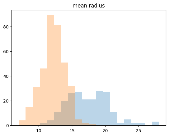

// 실습 코드
plt.figure(figsize=[20, 15])
for col in range(30):
  plt.subplot(8, 4, col+1)
  _, bins=np.histogram(cancer.data[:, 0], bins=20)

  plt.hist(malignant[:, 0], bins=bins, alpha=0.3)   # alpha: 투명도
  plt.hist(benign[:, 0], bins=bins, alpha=0.3)
  plt.title(cancer.feature_names[col])
  if col==0: plt.legend(cancer.target_names)
  plt.xticks([])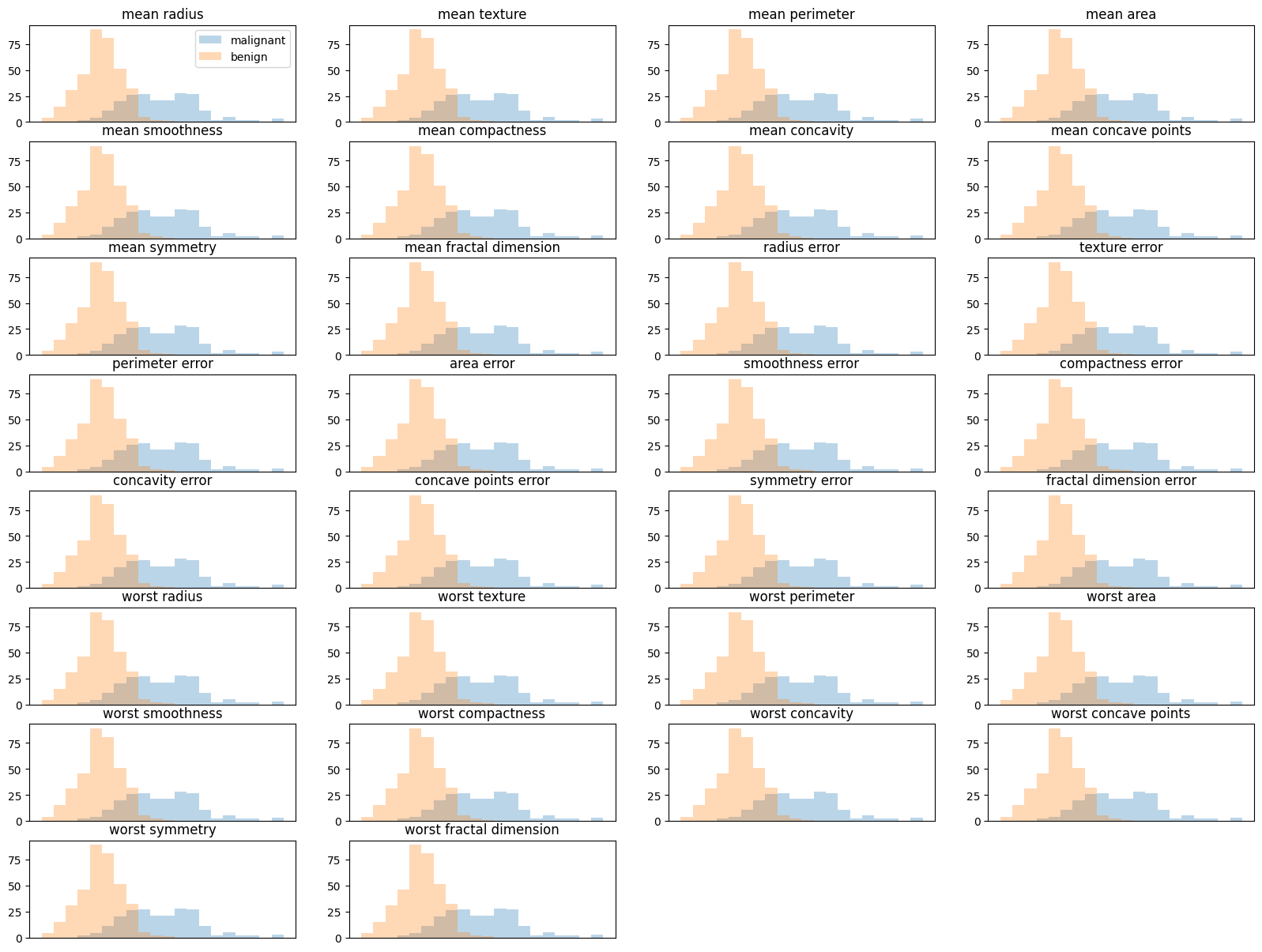

// 실습 코드
from sklearn.linear_model import LogisticRegression

scores = []

# iteration인 for문을 왜 돌렸는가? 비슷한 방법은 무엇일까?
# => 데이터 분할에 따른 성능 변화를 확인하기 위해, 비슷한 방법은 K-Fold Cross Validation
# 하지만 train_test_split를 해서 매번 랜덤하게 훈련/테스트 데이터가 분할하는데
# => 한번이라도 테스트데이터가 곂칠 수 도있으므로 좋은 방법은 아님

for i in range(10):
  X_train, X_test, y_train, y_test = train_test_split(cancer.data, cancer.target, test_size=0.2)

  model = LogisticRegression(max_iter = 5000)
  model.fit(X_train, y_train)

  score = model.score(X_test, y_test)
  scores.append(score)

print('scores =', scores)


# scores = [0.9473684210526315, 0.9736842105263158, 0.9824561403508771, 0.9122807017543859, 0.9473684210526315, 0.9473684210526315, 0.9473684210526315, 0.9736842105263158, 0.9649122807017544, 0.9736842105263158]

// 실습 코드
fig = plt.figure(figsize=[14, 14])
fig.suptitle('Breast Cancer - feature analysis', fontsize=20)

for col in range(cancer.feature_names.shape[0]):  # 30 features
  plt.subplot(8, 4, col+1)
  _, bins=np.histogram(cancer.data[:, col], bins=50)
  plt.hist(malignant[:, col], bins=bins, alpha=0.5, label='malignant', color='red')
  plt.hist(benign[:, col], bins=bins, alpha=0.5, label='benign', color='green')

  plt.title(cancer.feature_names[col]+('(%d)' %col))
  plt.xticks([])
  plt.yticks([])
  if col==0: plt.legend()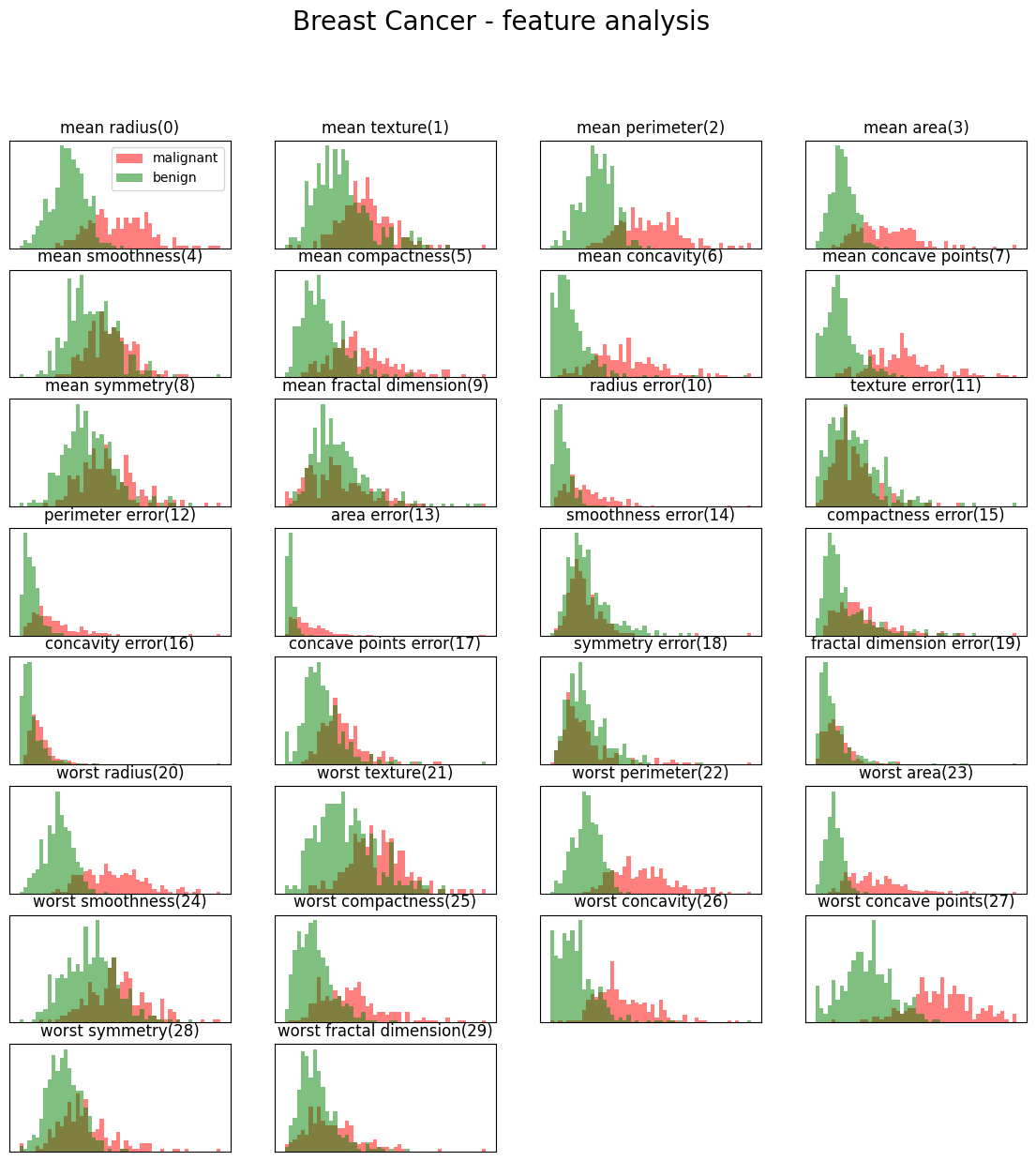

// 실습 코드
model.fit(X_train, y_train)

score = model.score(X_test, y_test)
scores.append(score)
print(moel.coef_) # 회귀계수
print(model.intercept_) # 절편
print(model.predict_proba(X_test))  # 예측(0, 1) 확률

예제: Kaggle - Mushroom Classification

// 실습 코드
import pandas as pd

mushroom = pd.read_csv('/content/drive/MyDrive/LG헬로비전_DX_School/250210/Mushroom Classification/mushrooms.csv')
mushroom

// 실습 코드
print(mushroom.info())  # 모든 column이 object -> encoder가 필요함.
print(mushroom['class'].unique()) # 중복을 제거한 것을 보자 # p, e

// 실습 코드
from sklearn.preprocessing import LabelEncoder
mush_encoded = mushroom.copy()
le = LabelEncoder()

for col in mush_encoded.columns:
  mush_encoded[col] = le.fit_transform(mush_encoded[col])

print(mush_encoded.head(10))
print(mush_encoded.columns)

// 실습 코드
import matplotlib.pyplot as plt
import seaborn as sns

plt.figure(figsize=(10, 10))
sns.heatmap(mush_encoded.corr(), cmap='inferno', square=True)
plt.show()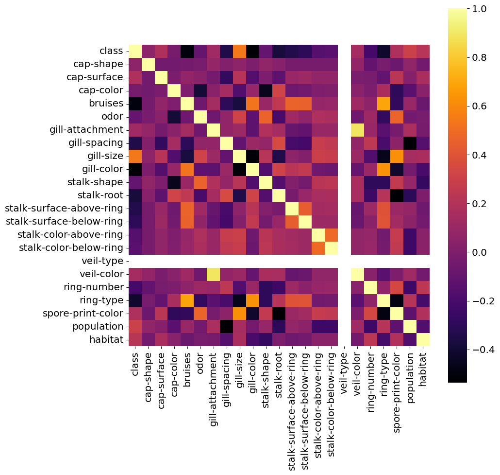

// 실습 코드
import matplotlib.pylab as pylab

params = {'legend.fontsize': 'x-large',
          'axes.labelsize': 'x-large',
          'axes.titlesize': 'x-large',
          'xtick.labelsize': 'x-large',
          'ytick.labelsize': 'x-large'}
pylab.rcParams.update(params)

// 실습 코드
def plot_col(col, hue=None, color=['blue', 'purple'], labels=None):
  fig, ax = plt.subplots(figsize=(15, 7))
  sns.countplot(x=col, hue=hue, palette=color, saturation=0.6, data=mush_encoded, dodge=True, ax=ax)
  ax.set(title=f"Mushroom {col.title()} Quantity", xlabel=f"{col.title()}", ylabel="Quantity")
  if labels != None:
    ax.set_xticklabels(labels)
  if hue != None:
    ax.legend(('Poisonous', 'Edible'), loc=0)

class_dict = ('Poisonous', 'Edible')
plot_col(col='class', labels=class_dict)
plt.show()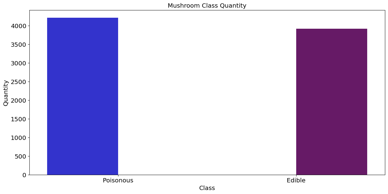

// 실습 코드
#Visualizing the number of mushrooms for each of the available cap sizes
shape_dict = {"bell":"b","conical":"c","convex":"x","flat":"f", "knobbed":"k","sunken":"s"}
labels = ('convex', 'bell', 'sunken', 'flat', 'knobbed', 'conical')
plot_col(col='cap-shape', hue='class', labels=labels)
plt.show()

// 실습 코드
import plotly.graph_objects as go

labels = ['Edible', 'Poison']
values = mush_encoded['class'].value_counts()

fig=go.Figure(data=[go.Pie(labels=labels, values=values)])
fig.update_traces(hoverinfo='label+percent', textinfo='value', textfont_size=20,
                  marker=dict(colors=['#87CEFA', '#7FFF00'],
                              line=dict(color='#FFFFFF',width=3)))
fig.show()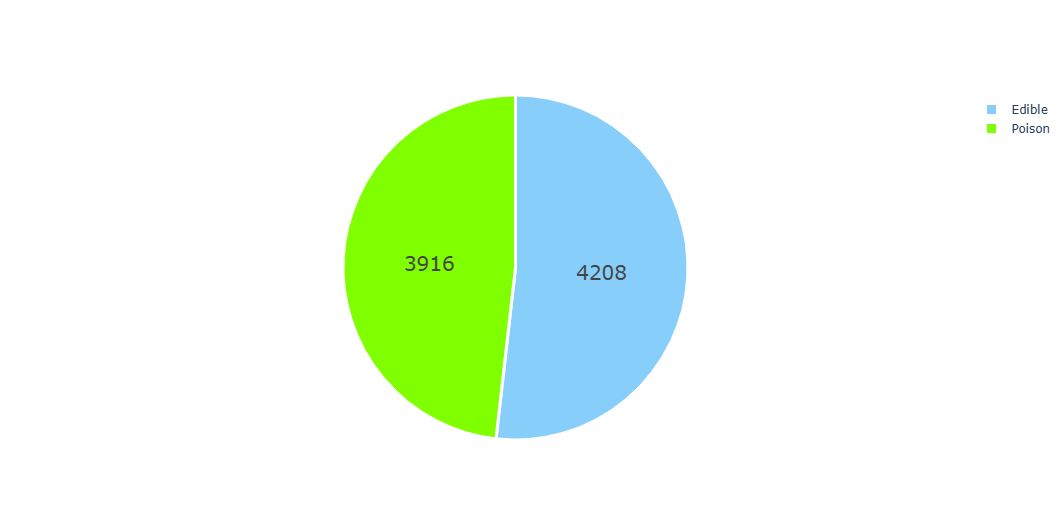

// 실습 코드
#Plot to understand the habitat of different mushrooms
labels = ['Woods', 'Grasses', 'Paths', 'Leaves', 'Urban', 'Meadows', 'Waste']
values = mush_encoded['habitat'].value_counts()
colors = ['#DEB887','#778899', '#B22222', '#FFFF00',
          '#F8F8FF','#FFE4C4','#FF69B4']

fig=go.Figure(data=[go.Pie(labels=labels,
                           values=values,
                           #marker_colors=labels,
                           pull=[0.1, 0, 0, 0, 0.2, 0, 0])])
fig.update_traces(title='Mushrooms Habitat Percentage',
                  hoverinfo='label+value',
                  textinfo='percent',
                  opacity=0.9,
                  textfont_size=20,
                  marker=dict(colors=colors,
                             line=dict(color='#000000', width=0.1)),
                 )
fig.show()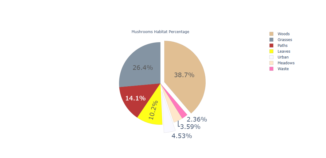

// 실습 코드
from sklearn.model_selection import train_test_split
from sklearn import preprocessing
import numpy as np

y = mush_encoded['class'].values
x = mush_encoded.drop(['class'], axis=1)
X_train, X_test, y_train,y_test = train_test_split(x, y, test_size=0.25, random_state=42)

from sklearn.linear_model import LogisticRegression
model_LR = LogisticRegression(solver='lbfgs', max_iter=1000)
model_LR.fit(X_train, y_train)

y_prob = model_LR.predict_proba(X_test)[:,1]  # 0하고 1(target) -> target -> 1
y_pred = np.where(y_prob > 0.5, 1, 0)  # 과적합을 유도함. target -> 1의 확율이 0.5 큰 경우는 1로 부여하고, 아닌 것은 0으로 부여한것.
# 강제로 0.5를 기준으로 잡힌 것은 아닌지?
# 기준값을 정한 것 자체가 상관은 없음.

model_LR.score(X_test, y_pred)

// 실습 코드
from sklearn.metrics import confusion_matrix, roc_auc_score, classification_report

confusion_matrix1 = confusion_matrix(y_test, y_pred)
confusion_matrix1

// 실습 코드
classification_report1 = classification_report(y_test, y_pred)
print(classification_report1)

// 실습 코드
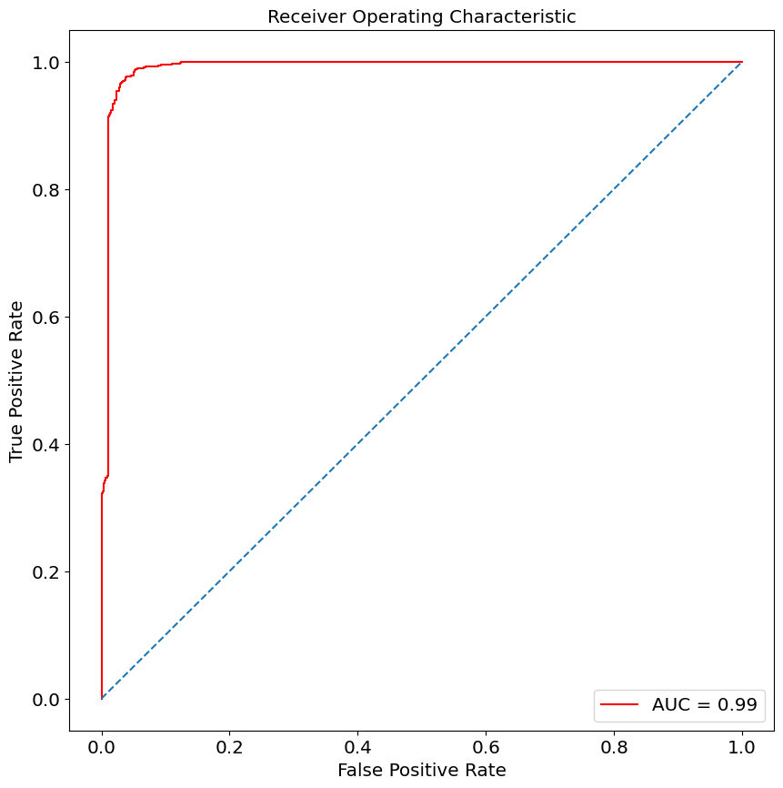
from sklearn.metrics import roc_curve, auc
false_positive_rate, true_positive_rate, thresholds = roc_curve(y_test, y_prob)
roc_auc = auc(false_positive_rate, true_positive_rate)
print(roc_auc)

plt.figure(figsize=(10, 10))
plt.title('Receiver Operating Characteristic')
plt.plot(false_positive_rate, true_positive_rate, color='red', label='AUC = %0.2f' % roc_auc)
plt.legend(loc = 'lower right')
plt.plot([0, 1], [0, 1], linestyle='--')
plt.axis('tight')
plt.ylabel('True Positive Rate')
plt.xlabel('False Positive Rate')

// 실습 코드
from sklearn.model_selection import train_test_split
from sklearn import preprocessing
import numpy as np

y = mush_encoded['class'].values
x = mush_encoded.drop(['class'], axis=1)
X_train, X_test, y_train,y_test = train_test_split(x, y, test_size=0.25, random_state=42)

from sklearn.linear_model import LogisticRegression
tuned_parameters = {'C':[0.001, 0.01, 0.1, 1, 10 , 100, 1000], 'penalty':['l1', 'l2']}
model_LR = LogisticRegression(solver='lbfgs', max_iter=1000)

from sklearn.model_selection import GridSearchCV
LR = GridSearchCV(model_LR, tuned_parameters, cv=10)
LR.fit(X_train, y_train)
y_prob = LR.predict_proba(X_test)[:, 1]
y_pred = np.where(y_prob > 0.5, 1, 0)

// 실습 코드
from sklearn.metrics import roc_curve, auc
false_positive_rate, true_positive_rate, thresholds = roc_curve(y_test, y_prob)
roc_auc = auc(false_positive_rate, true_positive_rate)
print(roc_auc)

plt.figure(figsize=(10, 10))
plt.title('Receiver Operating Characteristic')
plt.plot(false_positive_rate, true_positive_rate, color='red', label='AUC = %0.2f' % roc_auc)
plt.legend(loc = 'lower right')
plt.plot([0, 1], [0, 1], linestyle='--')
plt.axis('tight')
plt.ylabel('True Positive Rate')
plt.xlabel('False Positive Rate')