로지스틱 회귀(Logistic Regression)
데이터 로드 및 전처리
- pandas를 사용하여 데이터 로드
- LabelEncoder()를 사용해 범주형 데이터를 숫자로 변환
=> 데이터셋이 범주형(Categorical) 데이터로 이루어져 있기 때문에, Label Encoding을 사용하여 숫자로 변환
=> LabelEncoder()를 사용하여 각 컬럼의 값을 0, 1, 2, ... 형태로 변환
// 실습 코드
import pandas as pd

mushroom = pd.read_csv('/content/drive/MyDrive/LG헬로비전_DX_School/250210/Mushroom Classification/mushrooms.csv')

from sklearn.preprocessing import LabelEncoder
mush_encoded = mushroom.copy()
le = LabelEncoder()

for col in mush_encoded.columns:
  mush_encoded[col] = le.fit_transform(mush_encoded[col])

mush_encoded.head(10)
독립변수(X)와 종속변수(y) 분리
- y = mush_encoded['class']: 버섯이 독성인지 아닌지를 나타내는 라벨
- x = mush_encoded.drop(['class'], axis=1): 나머지 특성(Feature)들
데이터 분할
- train_test_split()을 이용해 75% 학습, 25% 테스트 데이터로 분할
=> 로지스틱 회귀(Logistic Regression) 모델을 생성
GridSearchCV를 사용해 최적의 C 값과 penalty 찾기 (cv=10 교차 검증)
- C: 로지스틱 회귀의 정규화 강도 (클수록 규제를 적게 함)
- penalty: L1(Lasso 정규화) 또는 L2(Ridge 정규화)를 적용할지 여부
// 실습 코드
#tuned model
from sklearn.linear_model import LogisticRegression
from sklearn.model_selection import cross_val_score, train_test_split
from sklearn import metrics
from sklearn import preprocessing
import numpy as np

y = mush_encoded['class'].values
x = mush_encoded.drop(['class'], axis=1)
X_train, X_test, y_train,y_test = train_test_split(x, y, test_size=0.25, random_state=42)

LR_model= LogisticRegression()

tuned_parameters = {'C': [0.001, 0.01, 0.1, 1, 10, 100, 1000] ,
              'penalty':['l1','l2']
                   }

from sklearn.model_selection import GridSearchCV

LR= GridSearchCV(LR_model, tuned_parameters,cv=10)
LR.fit(X_train,y_train)
// 실습 코드
print("하이퍼파라미터 : ", LR.best_params_)
y_prob = LR.predict_proba(X_test)[:, 1]
y_pred = np.where(y_prob > 0.5, 1, 0)
# 하이퍼파라미터 : {'C': 1000, 'penalty': 'l2'}최적 하이퍼파라미터 모델 학습 및 평가
- bestparams를 활용한 모델 재학습
- 예측 수행 및 accuracy, confusion_matrix, classification_report 출력
하이퍼파라미터 저장 및 불러오기
- JSON 파일 저장 및 불러오기
- Pickle 파일 저장 및 불러오기
// 실습 코드
# 파라미터 저장 -> JSON 파일로 저장
import json   # javascript object notation
from sklearn.linear_model import LogisticRegression

best_params = LR.best_params_

# 저장
with open('best_params.json', 'w') as f:
  json.dump(best_params, f)

# 불러오기
with open('/content/best_params.json', 'r') as f:
  best_params = json.load(f)

LR_model = LogisticRegression(C=best_params['C'], penalty=best_params['penalty'])
LR_model.fit(X_train, y_train)
y_pred = LR_model.predict(X_test)

from sklearn import metrics
accuracy = metrics.accuracy_score(y_test, y_pred)
print(f"Accuracy : {accuracy:.4f}")
print(metrics.confusion_matrix(y_test, y_pred))
print(metrics.classification_report(y_test, y_pred))


"""
Accuracy : 0.9572
[[988  52]
 [ 35 956]]
              precision    recall  f1-score   support

           0       0.97      0.95      0.96      1040
           1       0.95      0.96      0.96       991

    accuracy                           0.96      2031
   macro avg       0.96      0.96      0.96      2031
weighted avg       0.96      0.96      0.96      2031
"""
// 실습 코드
# 파라미터 저장 -> Pickle 파일로 저장
import pickle # 이진 직렬화 방식(이진화) => 객체를 직렬화하는 방법으로 사용됨
from sklearn.linear_model import LogisticRegression
# 저장
best_params = LR.best_params_
with open('/content/best_params.pkl', 'wb') as f:
pickle.dump(best_params, f)
# 불러오기
with open('best_params.pkl', 'rb') as f:
best_params = pickle.load(f)
LR_model = LogisticRegression(C=best_params['C'], penalty=best_params['penalty'])
LR_model.fit(X_train, y_train)
y_pred = LR_model.predict(X_test)
from sklearn import metrics
accuracy = metrics.accuracy_score(y_test, y_pred)
print(f"Accuracy : {accuracy:.4f}")
print(metrics.confusion_matrix(y_test, y_pred))
print(metrics.classification_report(y_test, y_pred))
"""
Accuracy : 0.9572
[[988 52]
[ 35 956]]
precision recall f1-score support
0 0.97 0.95 0.96 1040
1 0.95 0.96 0.96 991
accuracy 0.96 2031
macro avg 0.96 0.96 0.96 2031
weighted avg 0.96 0.96 0.96 2031
"""-
json : 데이터를 다른 시스템과 공유하거나 사람이 읽을 수 있게 쓰는 용도
-
pickle : 파이썬 객체(ex. 모델, 클래스 등)를 그대로 불러오고 싶으면 pickle이 적합
=> 파이썬에서 사용가능 함
의사결정트리(Decision Tree)
의사결정트리 모델 기본 적용
- DecisionTreeClassifier() 모델 학습 및 성능 평가 (accuracy 출력)
- tree.plot_tree()를 사용한 의사결정트리 시각화
// 실습 코드
import numpy as np
import pandas as pd
import matplotlib.pyplot as plt
from sklearn.datasets import load_iris
from sklearn.model_selection import train_test_split
from sklearn.tree import DecisionTreeClassifier

iris = load_iris()
X_train, X_test, y_train, y_test = train_test_split(iris.data, iris.target,
                                                    test_size=0.2, random_state=42)
# stratify : target
DT = DecisionTreeClassifier()
DT.fit(X_train, y_train)
print('accuracy : {:.2f}'.format(DT.score(X_test, y_test)))

from sklearn import tree

tree.plot_tree(DT)
plt.show()


# accuracy : 1.00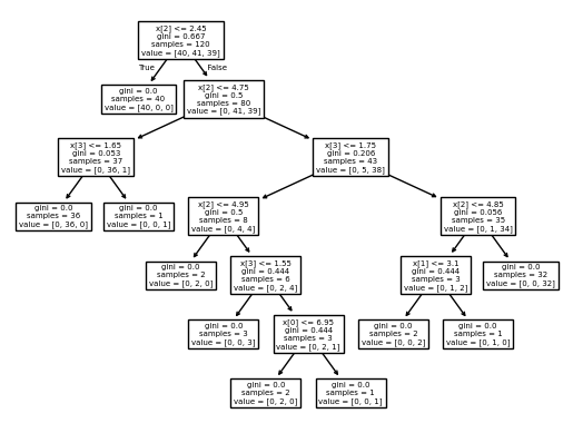
Graphviz를 활용한 트리 시각화
- export_graphviz()를 사용해 .dot 파일로 트리 저장 후 graphviz로 시각화
// 실습 코드
!pip install graphviz

from sklearn.tree import export_graphviz
from graphviz import Source

export_graphviz(DT, #모델
                out_file='iris_tree.dot', #저장경로 설정
                feature_names=iris.feature_names, #변수명
                class_names=iris.target_names, #종속변수
                rounded= True,
                filled=True)

Source.from_file('iris_tree.dot')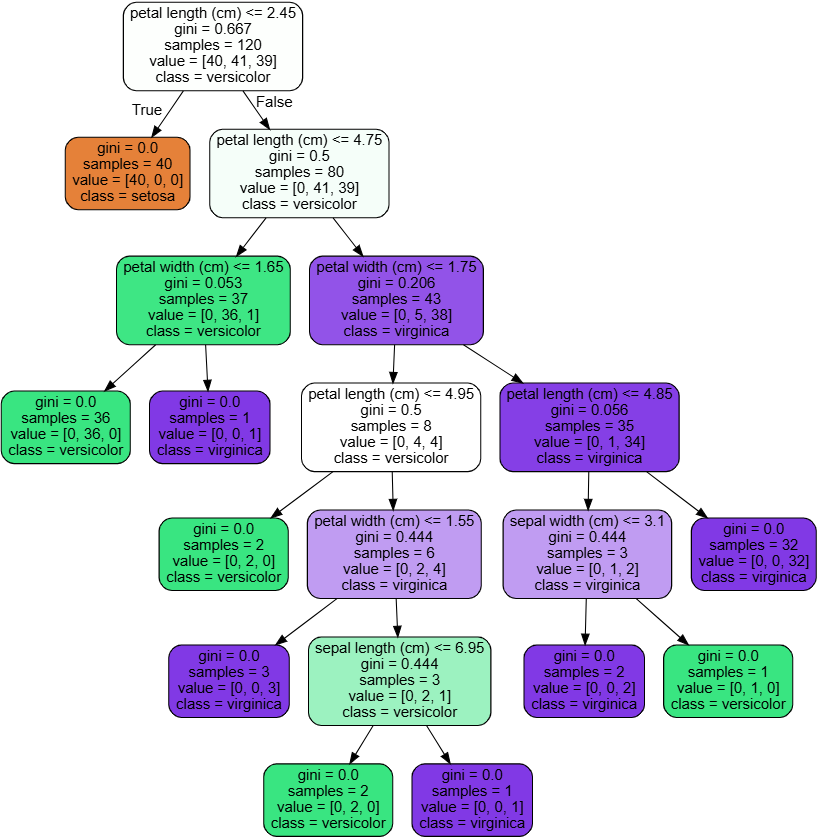
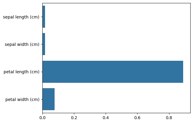
Feature Importance 분석
- featureimportances 속성을 사용해 변수 중요도 추출
- seaborn.barplot()을 이용해 변수 중요도 시각화
// 실습 코드
import seaborn as sns
# feature importance 추출     feature importance :  어떤 feature이 모델이 많이 봤는지
print("Feature importances:\n{0}".format(np.round(DT.feature_importances_, 3)))

# feature별 importance 매핑
for name, value, in zip(iris.feature_names, DT.feature_importances_):
  print('{0} : {1:.3f}'.format(name, value))

# feature importance를 column 별로 시각화 하기
sns.barplot(x=DT.feature_importances_ , y=iris.feature_names)

"""
Feature importances:
[0.017 0.017 0.889 0.077]
sepal length (cm) : 0.017
sepal width (cm) : 0.017
petal length (cm) : 0.889
petal width (cm) : 0.077
"""
기본 모델 학습 및 평가
- DecisionTreeClassifier() 모델 학습 및 성능 평가 (accuracy 출력)
- tree.plot_tree()를 사용해 의사결정트리 시각화
// 실습 코드
from sklearn.tree import DecisionTreeClassifier
from sklearn.datasets import load_breast_cancer
from sklearn.model_selection import train_test_split
from sklearn import tree

cancer = load_breast_cancer()
X_train, X_test, y_train, y_test = train_test_split(cancer.data, cancer.target,
                                                    stratify=cancer.target,
                                                    random_state=42)
clf = DecisionTreeClassifier()
clf.fit(X_train, y_train)
print('Accuracy on training set : {:.3f}'.format(clf.score(X_train, y_train)))
print('Accuracy on test set : {:.3f}'.format(clf.score(X_test, y_test)))

# Accuracy on training set : 1.000
# Accuracy on test set : 0.937
Feature Importance 분석 및 시각화
- featureimportances 속성을 사용해 변수 중요도 추출
- seaborn.barplot()을 활용한 변수 중요도 시각화
// 실습 코드
import numpy as np
import matplotlib.pyplot as plt

def plot_feature_importances_cancer(model):
  n_features = cancer.data.shape[1]
  plt.barh(np.arange(n_features), model.feature_importances_, align='center')
  plt.yticks(np.arange(n_features), cancer.feature_names)
  plt.xlabel("Feature importance")
  plt.ylabel("Feature")
  plt.ylim(-1, n_features)

plot_feature_importances_cancer(clf)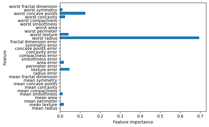
하이퍼파라미터 최적화 (GridSearchCV)
- 튜닝 대상 하이퍼파라미터
criterion: ['gini', 'entropy', 'log_loss']
max_depth, min_samples_split, min_samples_leaf, max_features, splitter - GridSearchCV를 활용해 최적의 하이퍼파라미터 탐색 후 모델 학습
// 실습 코드
from sklearn.tree import DecisionTreeClassifier
from sklearn.datasets import load_breast_cancer
from sklearn.model_selection import train_test_split, GridSearchCV
from sklearn import tree

cancer = load_breast_cancer()
X_train, X_test, y_train, y_test = train_test_split(cancer.data, cancer.target,
                                                    stratify=cancer.target,
                                                    random_state=42)
param_grid_extended = {
    'criterion':['gini', 'entropy', 'log_loss'],  # 분할 기준
    'max_depth':[None, 5, 10, 15, 20, 25, 30],  # 더 많은 깊은 트리 허용
    'min_samples_split':[2, 5, 10, 20, 50], # 노드 분할 최소 샘플 수 증가
    'min_samples_leaf':[1, 2, 5, 10, 20], # 리프 노드 최소 샘플 수 추가
    'max_features':[None, 'sqrt', 'log2'], # 사용할 특성 개수
    'splitter':['best', 'random'] # 데이터 분할 방식 추가
}

grid_search_extended = GridSearchCV(
    DecisionTreeClassifier(random_state=0),
    param_grid_extended,
    cv=5,
    scoring='accuracy',
    n_jobs= -1 # cpu = -1 -> total
)
# 최적의 하이퍼파라미터 확인
grid_search_extended.fit(X_train, y_train)
# 최적의 하이퍼파라미터로 모델 학습
best_params_extend = grid_search_extended.best_params_

best_clf_extended = DecisionTreeClassifier(**best_params_extend, random_state=0)  # 여러개의 튜플로 받는 건 *args, 딕셔너리로 받는 건 **kwargs
best_clf_extended.fit(X_train, y_train)

print('Accuracy on training set : {:.3f}'.format(best_clf_extended.score(X_train, y_train)))
print('Accuracy on test set : {:.3f}'.format(best_clf_extended.score(X_test, y_test)))

import numpy as np
import matplotlib.pyplot as plt

def plot_feature_importances_cancer(model):
  n_features = cancer.data.shape[1]
  plt.barh(np.arange(n_features), model.feature_importances_, align='center')
  plt.yticks(np.arange(n_features), cancer.feature_names)
  plt.xlabel("Feature importance")
  plt.ylabel("Feature")
  plt.ylim(-1, n_features)

plot_feature_importances_cancer(best_clf_extended)

# Accuracy on training set : 1.000
# Accuracy on test set : 0.944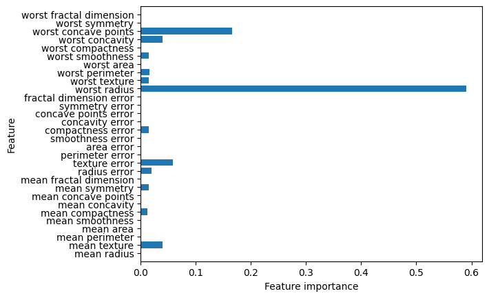
랜덤 포레스트 (Random Forest)
- 기본 모델 학습 및 평가
RandomForestClassifier()를 사용해 학습 및 성능 평가
// 실습 코드
# RandomForest 버전
from sklearn.ensemble import RandomForestClassifier
from sklearn.tree import DecisionTreeClassifier
from sklearn.datasets import load_breast_cancer
from sklearn.model_selection import train_test_split, GridSearchCV
from sklearn import tree

cancer = load_breast_cancer()
X_train, X_test, y_train, y_test = train_test_split(cancer.data, cancer.target,
                                                    stratify=cancer.target,
                                                    random_state=42)
하이퍼파라미터 최적화 (GridSearchCV)
- 튜닝 대상 하이퍼파라미터
n_estimators: [50, 100, 200, 300] (트리 개수)
criterion: ['gini', 'entropy', 'log_loss'] (분할 기준)
max_depth: [None, 10, 20, 30] (트리 깊이)
min_samples_split, min_samples_leaf, max_features, bootstrap
// 실습 코드
param_grid_extended = {
    'n_estimators':[50, 100, 200, 300], # 트리 개수
    'criterion':['gini', 'entropy', 'log_loss'],  # 분할 기준
    'max_depth':[None, 10, 20, 30],  # 트리 깊이
    'min_samples_split':[2, 5, 10], # 노드 분할 최소 샘플 수
    'min_samples_leaf':[1, 2, 5], # 리프 노드 최소 샘플 수
    'max_features':['sqrt', 'log2', None], # 사용할 특성 개수
    'bootstrap':[True, False]  # 부트스트랩 샘플링 여부
}

grid_search_extended = GridSearchCV(
    RandomForestClassifier(random_state=0),
    param_grid_extended,
    cv=5,
    scoring='accuracy',
    n_jobs= -1 # cpu = -1 -> total
)
# 최적의 하이퍼파라미터 확인
grid_search_extended.fit(X_train, y_train)
# 최적의 하이퍼파라미터로 모델 학습
best_params_extend = grid_search_extended.best_params_

best_clf_extended = RandomForestClassifier(**best_params_extend, random_state=0)  # 여러개의 튜플로 받는 건 *args, 딕셔너리로 받는 건 **kwargs
best_clf_extended.fit(X_train, y_train)

print('Accuracy on training set : {:.3f}'.format(best_clf_extended.score(X_train, y_train)))
print('Accuracy on test set : {:.3f}'.format(best_clf_extended.score(X_test, y_test)))

import numpy as np
import matplotlib.pyplot as plt
Feature Importance 분석 및 시각화
- featureimportances 속성을 활용한 변수 중요도 계산
- seaborn.barplot()을 사용해 중요도 시각화
// 실습 코드
def plot_feature_importances_cancer(model):
  n_features = cancer.data.shape[1]
  plt.barh(np.arange(n_features), model.feature_importances_, align='center')
  plt.yticks(np.arange(n_features), cancer.feature_names)
  plt.xlabel("Feature importance")
  plt.ylabel("Feature")
  plt.ylim(-1, n_features)

plot_feature_importances_cancer(best_clf_extended)


# Accuracy on training set : 1.000
# Accuracy on test set : 0.958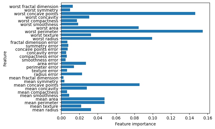
가우시안 나이브 베이즈(Gaussian Naive Bayes)
데이터 로드 및 전처리
- load_iris()를 사용해 데이터셋 로드
- 입력 데이터 X와 타겟 y 분리
// 실습 코드
import numpy as np
import pandas as pd
import matplotlib.pyplot as plt
import seaborn as sns
from sklearn.datasets import load_iris
from sklearn.model_selection import train_test_split, GridSearchCV
from sklearn.naive_bayes import GaussianNB  # gaussian: nomal
from sklearn.metrics import accuracy_score

data = load_iris()
X = data.data
y = data.target
feature = data.feature_names
하이퍼파라미터 최적화 (GridSearchCV)
- GaussianNB는 기본적으로 하이퍼파라미터 최적화가 필요하지 않지만, var_smoothing을 튜닝
- GridSearchCV를 사용해 최적의 var_smoothing 값 탐색
// 실습 코드
# 하이퍼파라미터 최적화 진행 -> GaussianNB는 하이퍼파라미터를 최적화 하지 않음.
# 강제로 하는 것
param_grid = {'var_smoothing':np.logspace(0, -9, num=100)}
gnb = GaussianNB()
grid_search = GridSearchCV(gnb, param_grid, cv=5, scoring='accuracy')
grid_search.fit(X, y)

best_gnb = grid_search.best_estimator_
y_pred = best_gnb.predict(X)
accuracy = accuracy_score(y, y_pred)
print('Best estimaters found', grid_search.best_params_)
print(f'model Accuracy : {accuracy : .4f}')
Feature Importance 분석 및 시각화
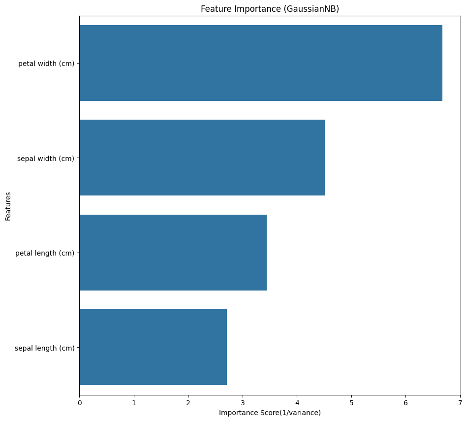
- GaussianNB는 분산이 작을수록 중요한 특성으로 간주되므로, 1/variance를 사용해 중요도 계산
- seaborn.barplot()을 활용한 변수 중요도 시각화
// 실습 코드
# Feature importance 계산(GaussianNB 기반)
# GaussianNB는 각 클래스별 평균(mu)과 분산(var)을 학습하므로, 분산이 작을수록 예측에 중요한 특성으로 간주할 수 있음(1/var 활용)
feature_importance = 1/(best_gnb.var_).mean(axis=0)  # 평균 분산의 역수를 중요도로 사용

# feature importance 시각화
importance_df = pd.DataFrame({'Feature' : feature, 'Importance' : feature_importance})
importance_df = importance_df.sort_values(by='Importance', ascending=False)

plt.figure(figsize=(10, 10))
sns.barplot(x="Importance", y="Feature", data=importance_df)
plt.title("Feature Importance (GaussianNB)")
plt.xlabel("Importance Score(1/variance)")
plt.ylabel('Features')
plt.show()

# Best estimaters found {'var_smoothing': 0.03511191734215131}
# model Accuracy :  0.9533