Bagging
- BaggingClassifier를 활용한 모델 학습
- GridSearchCV를 사용한 하이퍼파라미터 최적화
- 최적 모델을 활용한 예측 및 평가
// 실습 코드
# Bagging

from sklearn.ensemble import BaggingClassifier  # Bagging 앙상블 학습기
from sklearn.tree import DecisionTreeClassifier  # 기본 학습기로 사용할 결정 트리
from sklearn.datasets import load_breast_cancer  # 유방암 데이터셋 로드
from sklearn.model_selection import train_test_split, GridSearchCV  # 데이터 분할 및 하이퍼파라미터 탐색
from sklearn.metrics import accuracy_score  # 모델 성능 평가를 위한 정확도 지표
import numpy as np

# 1️. 데이터 로드 및 분할
cancer = load_breast_cancer()  # 유방암 데이터셋 로드

# 훈련 데이터와 테스트 데이터로 분리
X_train, X_test, y_train, y_test = train_test_split(
    cancer.data, cancer.target,
    stratify=cancer.target,  # 클래스 비율을 유지하도록 설정
    random_state=42  # 결과 재현성을 위한 랜덤 시드 고정
)

# 2️. Bagging 모델 설정
# 기본 학습기로 DecisionTreeClassifier 사용
base_dt = DecisionTreeClassifier(random_state=42)

# BaggingClassifier 생성 (결정 트리를 여러 개 앙상블로 학습)
bagging_clf = BaggingClassifier(estimator=base_dt, random_state=42)

# 3️. 하이퍼파라미터 탐색을 위한 설정 (GridSearchCV)
param_grid = {
    'n_estimators': [50, 100, 200, 300],  # 트리 개수 (모델 수)
    'max_samples': [0.5, 0.7, 1.0],  # 각 기본 모델이 학습할 샘플 비율
    'max_features': [0.5, 0.7, 1.0],  # 각 기본 모델이 학습할 특성(Feature) 개수 비율
}

# GridSearchCV 설정
grid_search = GridSearchCV(
    bagging_clf,  # BaggingClassifier 모델
    param_grid,  # 탐색할 하이퍼파라미터 조합
    cv=5,  # 5-Fold 교차 검증 수행
    scoring='accuracy',  # 평가 지표: 정확도 (accuracy)
    n_jobs=-1  # 병렬 처리 (CPU 전체 사용)
)

# 4️. 하이퍼파라미터 최적화 수행
grid_search.fit(X_train, y_train)  # 학습 데이터로 GridSearchCV 수행

# 5️. 최적 하이퍼파라미터 확인
best_params_extend = grid_search.best_params_  # 최적 하이퍼파라미터 출력
print("Best Parameters:", best_params_extend)

# 6️. 최적 모델을 사용하여 평가
best_model = grid_search.best_estimator_  # 최적 모델 가져오기
y_pred = best_model.predict(X_test)  # 테스트 데이터 예측 수행

# 모델 성능 평가 (Accuracy)
accuracy = accuracy_score(y_test, y_pred)
print('Test Accuracy:', accuracy)  # 테스트 정확도 출력

"""
Best Parameters: {'max_features': 0.7, 'max_samples': 0.7, 'n_estimators': 100}
Test Accuracy: 0.958041958041958
"""
피마 인디언 당뇨병 예측
데이터 소개
- Kaggle 데이터셋: Pima Indians Diabetes Database
- 북아메리카 피마 지역 원주민의 Type-2 당뇨병 여부를 예측하는 데이터
- 당뇨병 발생 원인은 주로 식습관 변화와 유전적 요인
- 서구화된 식습관 도입으로 인해 당뇨병 환자가 증가
데이터 변수 설명
- Pregnancies: 임신 횟수
- Glucose: 포도당 부하 검사 수치
- BloodPressure: 혈압(mm Hg)
- SkinThickness: 팔 삼두근 뒤쪽의 피하지방 측정값(mm)
- Insulin: 2시간 혈청 인슐린(mu U/ml)
- BMI: 체질량 지수
- DiabetesPedigreeFunction: 당뇨병 혈통 기능
- Age: 나이
- Outcome: 당뇨병 여부 (0: 음성, 1: 양성)
데이터 로드 및 기본 정보 확인
- 데이터셋을 불러오고, 클래스 불균형 여부 확인
- Outcome 클래스 비율을 분석하여 단순 정확도(Accuracy)만으로 모델 평가가 어려운지 판단
// 실습 코드
import numpy as np
import pandas as pd
import matplotlib.pyplot as plt

from sklearn.model_selection import train_test_split
from sklearn.metrics import accuracy_score, precision_score,recall_score,roc_auc_score
from sklearn.metrics import f1_score, confusion_matrix,precision_recall_curve, roc_curve
from sklearn.preprocessing import StandardScaler
from sklearn.linear_model import LogisticRegression
from sklearn.tree import DecisionTreeClassifier

diabetes_data = pd.read_csv('/content/drive/MyDrive/LG헬로비전_DX_School/250212/diabetes.csv')
print(diabetes_data['Outcome'].value_counts())
# 불균형 문제 -> acc만 보는 것은 신뢰하기 어려움. confusion matrix를 봐야함

"""
Outcome
0    500
1    268
Name: count, dtype: int64
"""
=> 데이터 불균형 문제 → Accuracy만으로 평가 어려움 → confusion matrix도 함께 확인해야 함
데이터 시각화 및 통계 분석
- 변수별 데이터 분포 분석 (히스토그램)
- Pregnancies, Glucose, BloodPressure 등 변수별 평균값 확인
// 실습 코드
diabetes_data['Pregnancies'].hist()
plt.show()
print('평균값 : {:.2f}'.format(diabetes_data['Pregnancies'].mean()))

diabetes_data['Glucose'].hist()
print('평균값 : {:.2f}'.format(diabetes_data['Glucose'].mean()))

diabetes_data['BloodPressure'].hist()
print('평균값 : {:.2f}'.format(diabetes_data['BloodPressure'].mean()))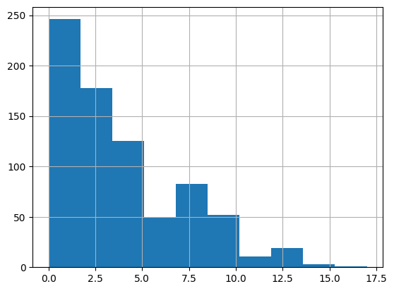
평균값 : 3.85
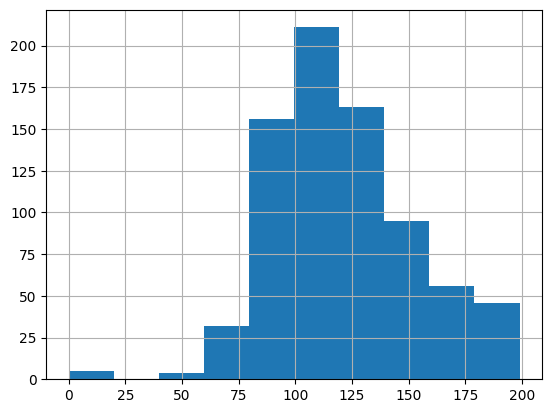
평균값 : 120.89
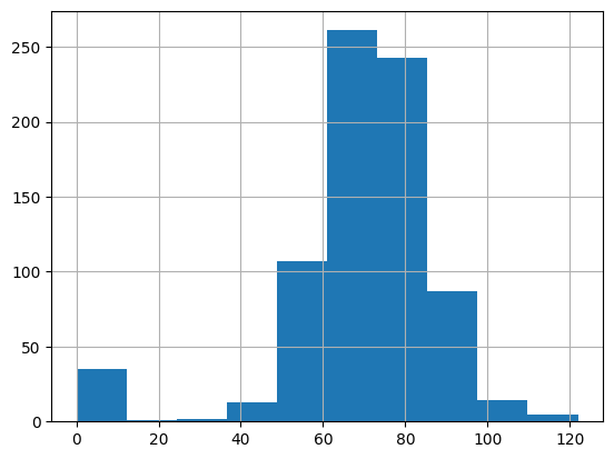
평균값 : 69.11
- 상관관계 분석 (Heatmap)
- 변수 간의 상관계수를 분석하여 상관관계가 높은 변수 탐색
// 실습 코드
import seaborn as sns

sns.heatmap(diabetes_data.corr(method='pearson'), annot=True)    # 피어슨 -> 연속형, 스피어만 -> 이산, 연속 둘다 가능
plt.show()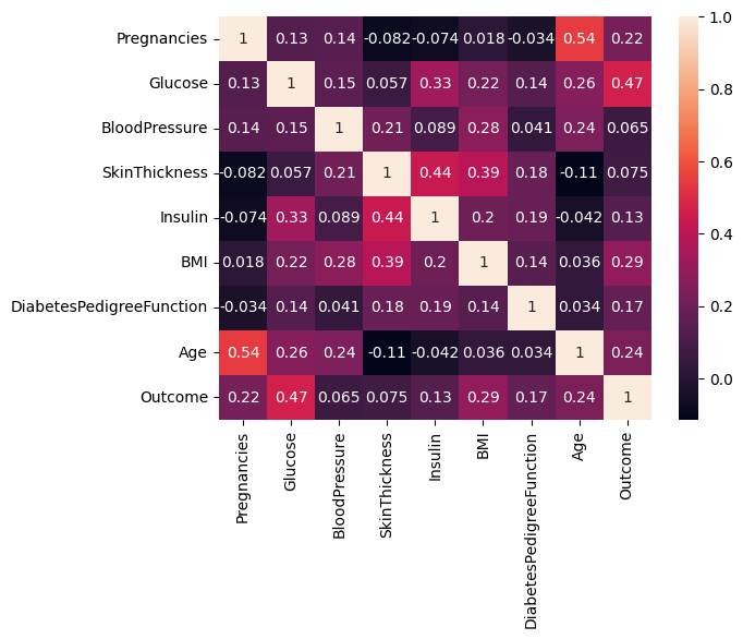
- 변수 간 관계 시각화 (Pairplot)
// 실습 코드
sns.pairplot(diabetes_data)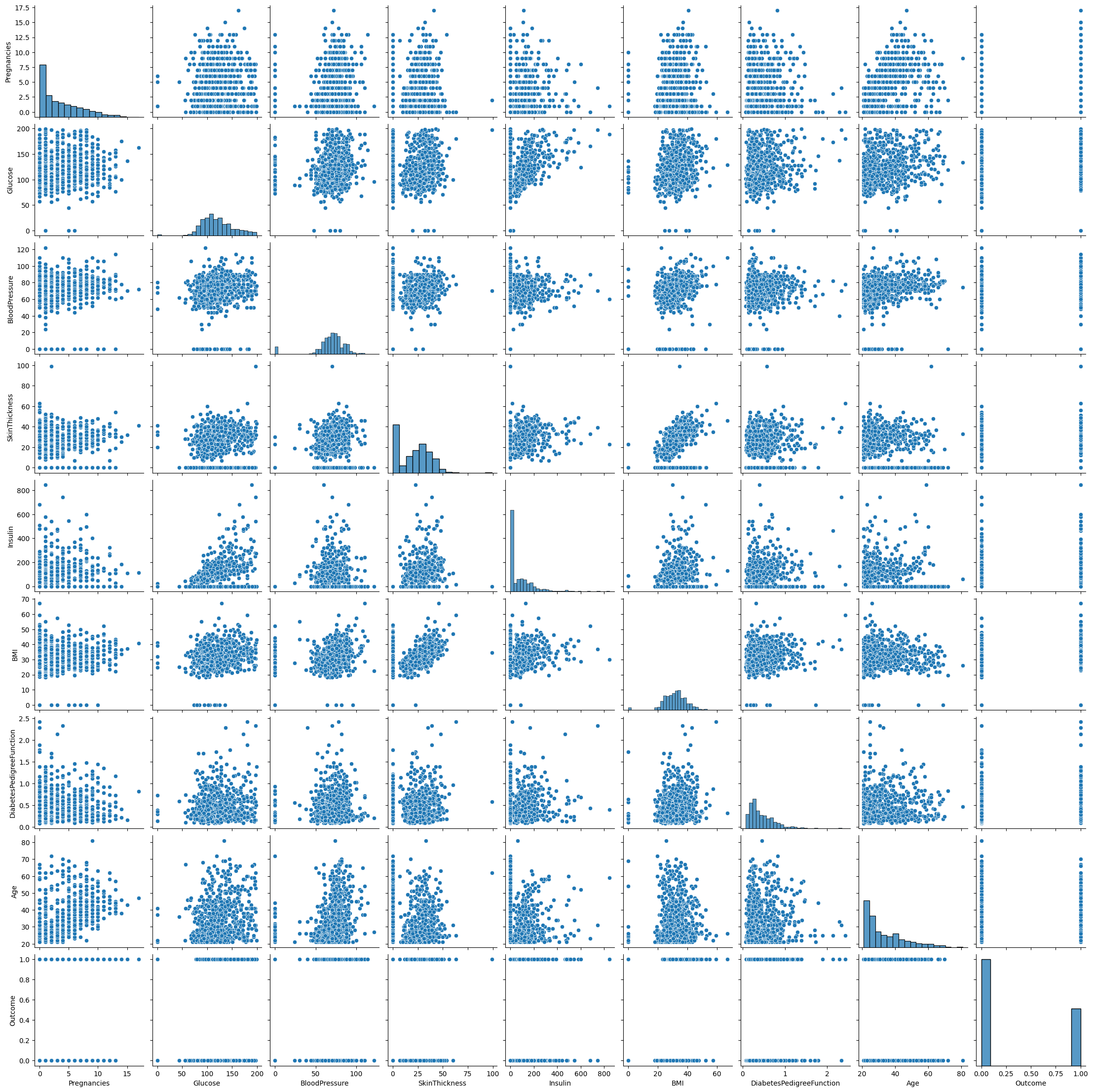
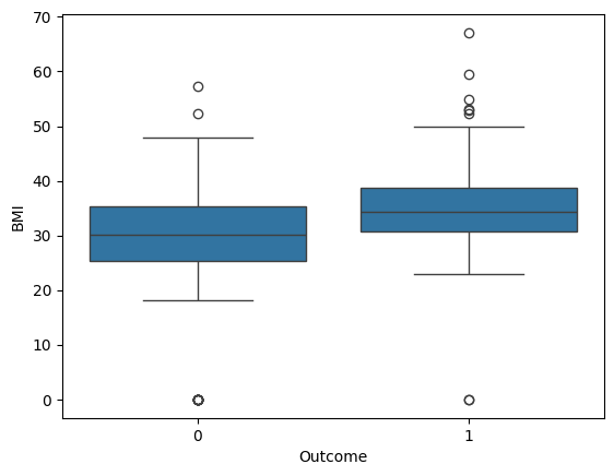
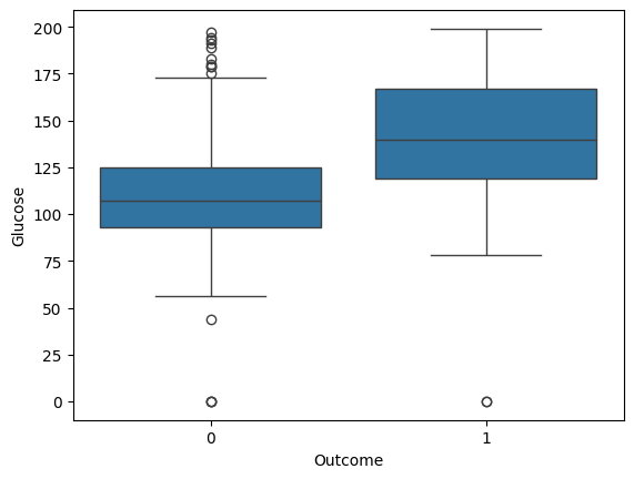
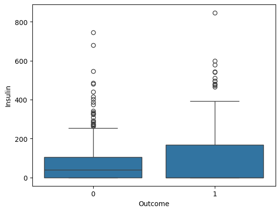
- 박스플롯을 활용한 변수별 당뇨병 영향 분석
- 주요 변수인 Pregnancies, BMI, Glucose, Insulin 값이 Outcome에 따라 차이가 나는지 확인
// 실습 코드
sns.boxplot(x='Outcome', y='Pregnancies', data=diabetes_data)
# 임신 횟수가 적을수록 당뇨병 발병이 적을 것이다.

sns.boxplot(x='Outcome', y='BMI', data=diabetes_data)
# BMI가 낮으면 당뇨병 발병이 적을 것이다. -> BMI식이 뭐지? -> 우리나라 계산방법과 다를 것이다.

sns.boxplot(x='Outcome', y='Glucose', data=diabetes_data)

sns.boxplot(x='Outcome', y='Insulin', data=diabetes_data)
# Outcome이 1인 부분은 왜 중위수가 안보이는가? -> 위 또는 아래에 붙어있을 것으로 예상(Q3 또는 Q1)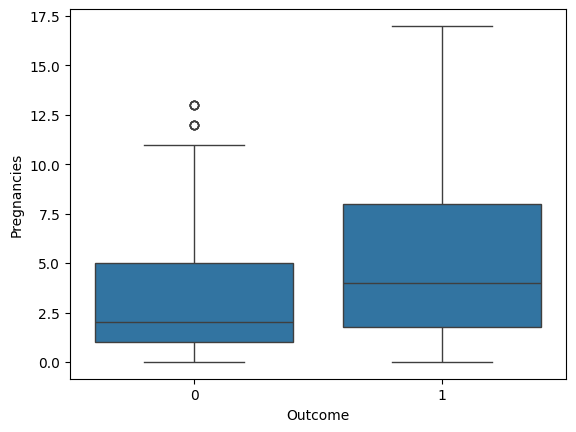
- 연령 및 임신 횟수에 따른 발병 여부 분석 (barplot 활용)
// 실습 코드
# 나이대별 발병 여부는 다를까?
sns.barplot(x='Age', y='Outcome', data=diabetes_data)
plt.show()

# -> 나이대에서 값이 고르게 분포되어 있으면 신뢰구간이 좁고,
#    나이대가 고르게 분포되어 있지 않으면 신뢰구간이 넓음.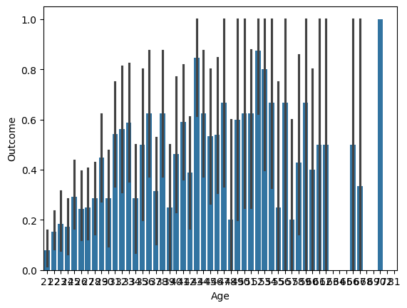
// 실습 코드
plt.figure(figsize=(12, 6))
sns.barplot(x='Pregnancies', y='Outcome', data=diabetes_data)
plt.show()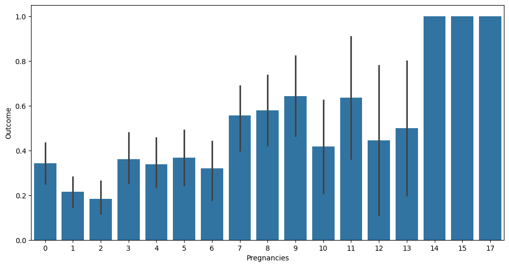
데이터 전처리
- 결측치 확인
- isna().sum()을 활용하여 결측치 여부 확인
// 실습 코드
print(diabetes_data.isna().sum())

# 결측치는 없음- 이상치 탐지 및 제거 (3-sigma 활용)
// 실습 코드
# Outlier Detection -> IQR9interquantile range), 3-sigma 사용
# 구간 벗어나는 값들을 삭제하려고 함
cols = diabetes_data.columns
for col in cols:
  mean = diabetes_data[col].mean()
  std = diabetes_data[col].std()
  threshold = mean + 3 * std
  n_outlier = np.sum(diabetes_data[col] > threshold)
  print(col + 'num of outlier:' + str(n_outlier))

# 0보다 작은 값들이 없으므로 3-sigma로도 충분함

"""
Pregnanciesnum of outlier:4
Glucosenum of outlier:0
BloodPressurenum of outlier:0
SkinThicknessnum of outlier:1
Insulinnum of outlier:18
BMInum of outlier:3
DiabetesPedigreeFunctionnum of outlier:11
Agenum of outlier:5
Outcomenum of outlier:0
"""- 0값 처리 (평균값 대체)
- Glucose, BloodPressure, SkinThickness, Insulin, BMI에서 0값을 평균값으로 대체
// 실습 코드
cols = diabetes_data.columns
for col in cols:
  mean = diabetes_data[col].mean()
  std = diabetes_data[col].std()
  threshold = mean + 3 * std
  diabetes_data.drop(diabetes_data[diabetes_data[col]>threshold].index[:],inplace=True)
diabetes_data.dropna()
print('after drop outlier:{}'.format(diabetes_data.shape))

# after drop outlier:(706, 9)
모델 학습 및 평가
- 데이터셋 분할
- train_test_split을 사용하여 학습 데이터와 테스트 데이터로 분리
// 실습 코드
X = diabetes_data.iloc[:, :-1]
y = diabetes_data.iloc[:, -1]

X_train, X_test, y_train, y_test = train_test_split(X, y, test_size=0.2, random_state=42, stratify=y)- 로지스틱 회귀 모델 학습
- LogisticRegression을 사용하여 모델 학습
- liblinear solver 적용
// 실습 코드
lr_clf = LogisticRegression(solver = 'liblinear')
lr_clf.fit(X_train,y_train)
pred = lr_clf.predict(X_test)
pred_proba = lr_clf.predict_proba(X_test)- 모델 평가
- 평가 함수(get_clf_eval) 정의
- confusion_matrix, accuracy_score, precision_score, recall_score, f1_score, roc_auc_score 활용
// 실습 코드
def get_clf_eval(y_test=None, pred=None):
  confusion = confusion_matrix(y_test, pred)
  accuracy = accuracy_score(y_test, pred)
  precision = precision_score(y_test, pred)
  recall = recall_score(y_test, pred)
  f1 = f1_score(y_test, pred)
  # ROC-AUROC 추가
  roc_auc = roc_auc_score(y_test, pred)
  print('오차 행렬')
  print(confusion)
  # ROC-AUROC print 추가
  print('정확도: {0:.4f}, 정밀도: {1:.4f}, 재현율: {2:.4f}, F1: {3:.4f}, AUC:{4:.4f}'.format(accuracy, precision, recall, f1, roc_auc))
get_clf_eval(y_test,pred)


"""
오차 행렬
[[83 12]
 [19 28]]
정확도: 0.7817, 정밀도: 0.7000, 재현율: 0.5957, F1: 0.6437, AUC:0.7347
"""- classification_report를 활용한 모델 성능 분석
// 실습 코드
from sklearn.metrics import classification_report

print(classification_report(y_test, pred))

# f1_score -> 정밀도, 민감도(재현율) -> 조화평균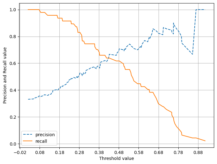
# 재현율이 낮음. -> threshold -> recall -> 강화를 해줄 수 있음- 정밀도-재현율 곡선 시각화
- precision_recall_curve_plot을 활용하여 threshold 값에 따른 Precision & Recall 변화 시각화
// 실습 코드
def precision_recall_curve_plot(y_test=None, pred_proba_c1=None):
  precisions, recalls, thresholds = precision_recall_curve(y_test, pred_proba_c1)

  # X축을 threshold값으로, Y축은 정밀도, 재현율 값으로 각각 Plot 수행. 정밀도는 점선으로 표시
  plt.figure(figsize=(8, 6))
  threshold_boundary = thresholds.shape[0]
  plt.plot(thresholds, precisions[0:threshold_boundary], linestyle='--', label='precision')
  plt.plot(thresholds, recalls[0:threshold_boundary], label='recall')

  # threshold 값 X축의 Scale을 0, 1 단위로 변경
  start, end = plt.xlim()
  plt.xticks(np.round(np.arange(start, end, 0.1), 2))

  # x축, y축 label과 legend, grid 설정
  plt.xlabel('Threshold value'); plt.ylabel('Precision and Recall value')
  plt.legend(); plt.grid()
  plt.show()

pred_proba_c1 = lr_clf.predict_proba(X_test)[:, 1]
precision_recall_curve_plot(y_test, pred_proba_c1)


"""
              precision    recall  f1-score   support

           0       0.81      0.87      0.84        95
           1       0.70      0.60      0.64        47

    accuracy                           0.78       142
   macro avg       0.76      0.73      0.74       142
weighted avg       0.78      0.78      0.78       142
"""
임계값 조정 및 성능 개선
- 0값 처리 (평균값 대체)
- Glucose, BloodPressure, SkinThickness, Insulin, BMI 변수에서 0값을 평균값으로 대체
// 실습 코드
zero_features = ['Glucose', 'BloodPressure', 'SkinThickness', 'Insulin', 'BMI']
total_count = diabetes_data['Glucose'].count()

for feature in zero_features:
  zero_count = diabetes_data[diabetes_data[feature] == 0][feature].count()
  print('{0} 0 건수는 {1}, 퍼센트는 {2:.2f} %'.format(feature, zero_count, 100*zero_count/total_count))

# zero_feature 리스트 내부에 저장된 개별 피쳐들에 대해서 0값을 평균값으로 대체
diabetes_data[zero_features] = diabetes_data[zero_features].replace(0, diabetes_data[zero_features].mean())
print('after drop outlier : {}'.format(diabetes_data.shape))


"""
Glucose 0 건수는 0, 퍼센트는 0.00 %
BloodPressure 0 건수는 0, 퍼센트는 0.00 %
SkinThickness 0 건수는 0, 퍼센트는 0.00 %
Insulin 0 건수는 0, 퍼센트는 0.00 %
BMI 0 건수는 0, 퍼센트는 0.00 %
after drop outlier : (706, 9)
"""- 데이터 정규화 (StandardScaler)
- StandardScaler를 적용하여 데이터 정규화
// 실습 코드
X = diabetes_data.iloc[:, :-1]
y = diabetes_data.iloc[:, -1]

scaler = StandardScaler()
X_scaled = scaler.fit_transform(X)
X_train, X_test, y_train, y_test = train_test_split(X_scaled, y, test_size = 0.2, random_state = 156, stratify=y)

lr_clf = LogisticRegression()
lr_clf.fit(X_train , y_train)
pred = lr_clf.predict(X_test)
get_clf_eval(y_test , pred)

"""
오차 행렬
[[88  7]
 [21 26]]
정확도: 0.8028, 정밀도: 0.7879, 재현율: 0.5532, F1: 0.6500, AUC:0.7398
"""- 임계값 조정 및 성능 비교
- Binarizer를 활용하여 여러 threshold 값을 적용 후 성능 비교
// 실습 코드
# Binarizer : 연속형 변수의 이항 변수화(binarization)
from sklearn.preprocessing import Binarizer

def get_eval_by_threshold(y_test, pred_proba_c1, thresholds):
  for custom_threshold in thresholds:
    binarizer = Binarizer(threshold=custom_threshold).fit(pred_proba_c1)
    custom_predict = binarizer.transform(pred_proba_c1)
    print('임계값:', custom_threshold)
    get_clf_eval(y_test, custom_predict)

thresholds = [0.3, 0.33, 0.36, 0.39, 0.42, 0.45, 0.48, 0.50]
pred_proba = lr_clf.predict_proba(X_test)
get_eval_by_threshold(y_test, pred_proba[:, 1].reshape(-1, 1), thresholds)


"""
임계값: 0.3
오차 행렬
[[75 20]
 [12 35]]
정확도: 0.7746, 정밀도: 0.6364, 재현율: 0.7447, F1: 0.6863, AUC:0.7671
임계값: 0.33
오차 행렬
[[78 17]
 [14 33]]
정확도: 0.7817, 정밀도: 0.6600, 재현율: 0.7021, F1: 0.6804, AUC:0.7616
임계값: 0.36
오차 행렬
[[81 14]
 [15 32]]
정확도: 0.7958, 정밀도: 0.6957, 재현율: 0.6809, F1: 0.6882, AUC:0.7667
임계값: 0.39
오차 행렬
[[82 13]
 [18 29]]
정확도: 0.7817, 정밀도: 0.6905, 재현율: 0.6170, F1: 0.6517, AUC:0.7401
임계값: 0.42
오차 행렬
[[84 11]
 [19 28]]
정확도: 0.7887, 정밀도: 0.7179, 재현율: 0.5957, F1: 0.6512, AUC:0.7400
임계값: 0.45
오차 행렬
[[86  9]
 [20 27]]
정확도: 0.7958, 정밀도: 0.7500, 재현율: 0.5745, F1: 0.6506, AUC:0.7399
임계값: 0.48
오차 행렬
[[87  8]
 [21 26]]
정확도: 0.7958, 정밀도: 0.7647, 재현율: 0.5532, F1: 0.6420, AUC:0.7345
임계값: 0.5
오차 행렬
[[88  7]
 [21 26]]
정확도: 0.8028, 정밀도: 0.7879, 재현율: 0.5532, F1: 0.6500, AUC:0.7398
"""