개요
Kaggle에서 주관하는 2024 Kaggle Playground Series Season 4, Episode 1
https://www.kaggle.com/competitions/playground-series-s4e1?rvi=1

원본 데이터
Bank Customer Churn Prediction

목표
은행 고객 이탈 예측
이진 분류 문제
데이터 소개
Customer ID : 각 고객의 고유 식별자
Surname : 고객의 성
Credit Score : 고객의 신용 점수를 나타내는 값
Geography : 고객이 거주하는 국가(프랑스, 스페인 또는 독일)
Gender : 고객의 성별
Age : 고객의 연령
Tenure : 고객 은행 이용 기간(년)
Balance : 고객의 계좌 잔고
NumOfProducts : 고객이 사용하는 은행 상품 수(예: 저축 계좌, 신용 카드)
HasCrCard : 고객의 신용 카드 보유 여부(1 = 예, 0 = 아니오)
IsActiveMember : 고객 활동 여부(1 = 예, 0 = 아니오)
EstimatedSalary : 고객 추정 급여
Exited : 고객이 이탈 여부(1 = 예, 0 = 아니오)
Feature Engineering
def drop_useless(df):
    df.drop(['id', 'CustomerId', 'Surname'], axis=1, inplace=True)
    return df

drop_useless(train)
drop_useless(origin)
drop_useless(test)

# train과 원본 데이터 병합
train = pd.concat([train, origin], ignore_index=True)

# 중복 열 제거
train.drop_duplicates(inplace=True)

# 각 열의 최빈값(mode)을 구하고 이를 딕셔너리에 저장
mode_values_train = train.mode().iloc[0]

# 각 열의 결측치를 해당 열의 최빈값으로 대체
train.fillna(mode_values_train, inplace=True)

# test에 대해서 동일하게 적용
mode_values_test = test.mode().iloc[0]
test.fillna(mode_values_test, inplace=True)

# 수치형 데이터를 구분 후 각각의 변수에 저장
# train과 test 두 데이터에 대해 각각 적용
num_cols = list(train.select_dtypes(exclude=['object']).columns)

num_cols_test = list(test.select_dtypes(exclude=['object']).columns)

# Encoding이 필요하지 않은 경우 저장하지 않음
num_cols = [col for col in num_cols if col not in ['Exited', 'IsActiveMember', 'HasCrCard']]
num_cols_test = [col for col in num_cols_test if col not in ['Exited', 'IsActiveMember', 'HasCrCard']]

# Gender Encoding
labelencoder = LabelEncoder()
train['Gender']=labelencoder.fit_transform(train['Gender'])
test['Gender']=labelencoder.fit_transform(test['Gender'])

# Geography OneHotEncoding
train = pd.get_dummies(train, columns=['Geography'])
test = pd.get_dummies(test, columns=['Geography'])
Standard Scaler 사용
# StandardScaler를 통해 수치형 데이터를 표준화
scaler = StandardScaler()
train[num_cols] = scaler.fit_transform(train[num_cols])
test[num_cols_test] = scaler.transform(test[num_cols_test])
MinMax Scaler 사용
# MinMaxScaler 통해 수치형 데이터를 표준화
scaler = MinMaxScaler()
train[num_cols] = scaler.fit_transform(train[num_cols])
test[num_cols_test] = scaler.transform(test[num_cols_test])
MinMax Scaler가 조금 더 높은 성능을 보임
Model Building
모델 선택
Catboost / XGBoost / LGBM 세 가지 모델 비교
ROC Curve
xgb = XGBClassifier()
cb = CatBoostClassifier()
lg = LGBMClassifier()

xgb.fit(X_train, y_train)
cb.fit(X_train, y_train)
lg.fit(X_train, y_train)

y_score_xgb = xgb.predict_proba(X_valid)[:, 1]
y_score_cb = cb.predict_proba(X_valid)[:, 1]
y_score_lg = lg.predict_proba(X_valid)[:, 1]

fpr_xgb, tpr_xgb, _ = roc_curve(y_valid, y_score_xgb)
roc_auc_xgb = auc(fpr_xgb, tpr_xgb)

fpr_cb, tpr_cb, _ = roc_curve(y_valid, y_score_cb)
roc_auc_cb = auc(fpr_cb, tpr_cb)

fpr_lg, tpr_lg, _ = roc_curve(y_valid, y_score_lg)
roc_auc_lg = auc(fpr_lg, tpr_lg)

plt.figure(figsize=(8, 6))
plt.plot(fpr_xgb, tpr_xgb, color='blue', lw=2, label='XGBoost (AUC = %0.2f)' % roc_auc_xgb)
plt.plot(fpr_cb, tpr_cb, color='red', lw=2, label='CatBoost (AUC = %0.2f)' % roc_auc_cb)
plt.plot(fpr_lg, tpr_lg, color='green', lw=2, label='LightGBM (AUC = %0.2f)' % roc_auc_lg)

plt.plot([0, 1], [0, 1], color='black', lw=2, linestyle='--')
plt.xlim([0.0, 1.0])
plt.ylim([0.0, 1.05])
plt.xlabel('False Positive Rate')
plt.ylabel('True Positive Rate')
plt.title('Receiver Operating Characteristic (ROC) Curve')
plt.legend(loc='lower right')
plt.show()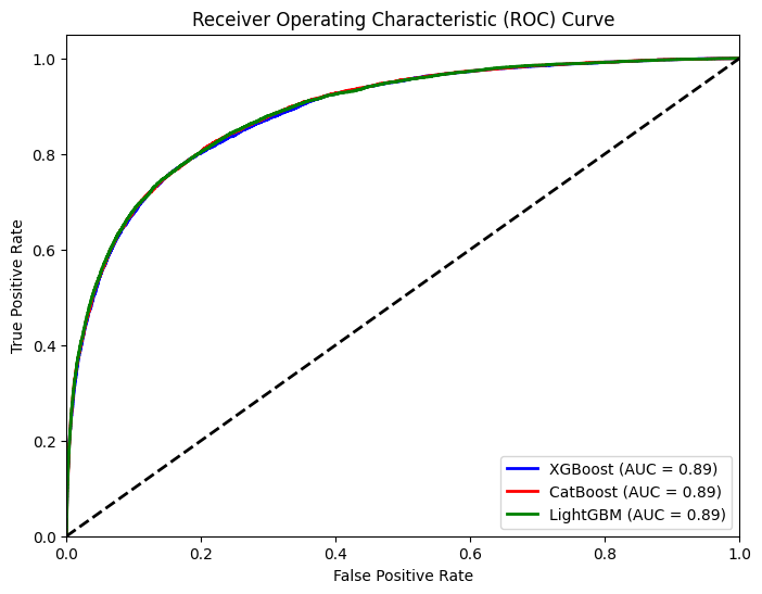
각 모델의 성능 차이는 매우 적게 나타남
제출을 통한 비교

4 - CatBoost
5 - XGBoost
6 - LGBM
LGBM이 가장 높은 결과를 보여줬기 때문에 LGBM으로 진행
1. predict를 통한 결과 확인
Grid Search를 통해 하이퍼파라미터 튜닝을 한 결과 미세하게 성능을 향상시킬 수 있었음

하지만 다른 사람들에 비해 낮은 정확도를 보였기 때문에 개선이 요구됨
2. predict_proba를 통한 결과 확인
예측을 하고 제출 할 때, 다른 사람들은 0과 1로만 제출하는 것이 아닌 .predict_proba() 값을 그대로 제출하는 것을 확인
위 방법 그대로 진행한 결과 약 10% 높은 결과를 확인할 수 있었음

