[Kaggle Competition]Multi-Class Prediction of Obesity Risk

조민서·2024년 2월 23일

Kaggle Competition

목록 보기

1/2

개요

Kaggle에서 주관하는 2024 Kaggle Playground Series Season 4, Episode 2
Multi-Class Prediction of Obesity Risk

원본 데이터
Obesity or CVD risk (Classify/Regressor/Cluster) 에서 데이터를 가져옴

목표

다양한 요인을 통해 NObeyesdad(비만도) 예측
NObeyesdad는

Insufficient_Weight
Normal_Weight
Overweight_Level_I
Overweight_Level_II
Obesity_Type_I
Obesity_Type_II
Obesity_Type_III

총 7단계로 구분

데이터 소개

id - 고유 id / int64
NObeyesdad - 비만도 / object
Gender - 성별 / object
Age - 나이 / float64
Height - 키 / float64
Weight - 몸무게 / float64
family_history_with_overweight - 가족 중 과체중 인원 여부 / object
FAVC - 고열량 음식 섭취 여부 / object
FCVC - 야채 섭취 빈도 / float64
NCP - 식사 빈도 / float64
CAEC - 식사 외 음식 섭취 빈도 / object
SMOKE - 흡연 여부 / object
CH2O - 수분 섭취 빈도 / float64
SCC - 칼로리 소비 모니터링 여부 / object
FAF - 활동 빈도 / float64
TUE - 전자기기 사용 빈도 / float64
CALC - 알코올 섭취 빈도 / object
MTRANS - 주로 사용하는 교통 수단 / object

EDA

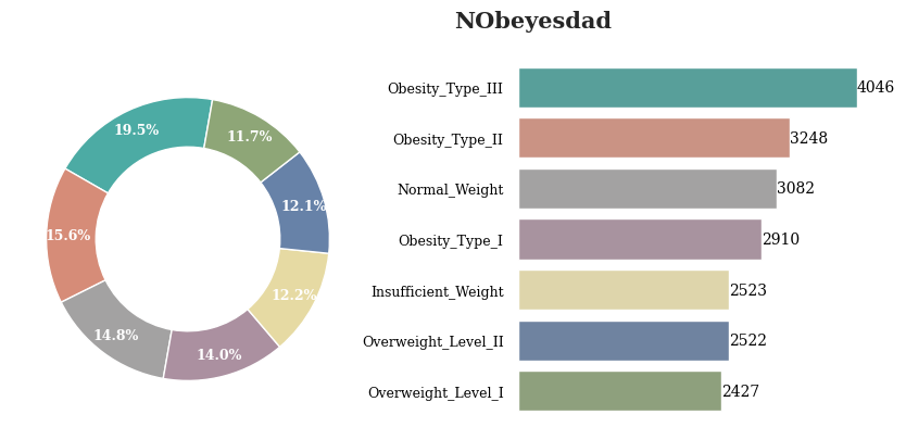
Obesity_Type_III가 가장 많은 것을 확인 할 수 있음
전체적으로 분포가 고르게 나타남

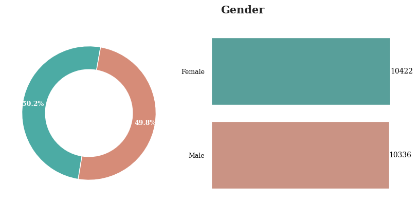
성별의 경우 남성이 미세하기 많지만 두 값의 비율은 차이가 없다고 할수 있음

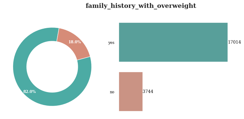
가족 중 과체중인 사람이 있는 경우는 대부분의 레코드에 대해서 yes로 나타남

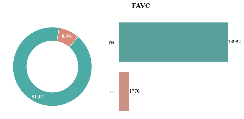
대부분의 레코드에 대해서 고열량 음식 섭취 여부는 yes로 나타남

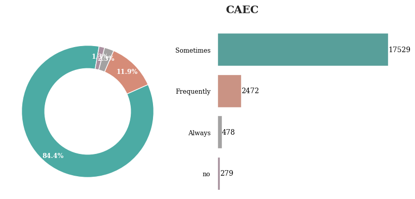
식사 외 음식을 섭취하는 빈도는 Sometimes가 가장 높게 나타났고, no가 가장 낮게 나타남

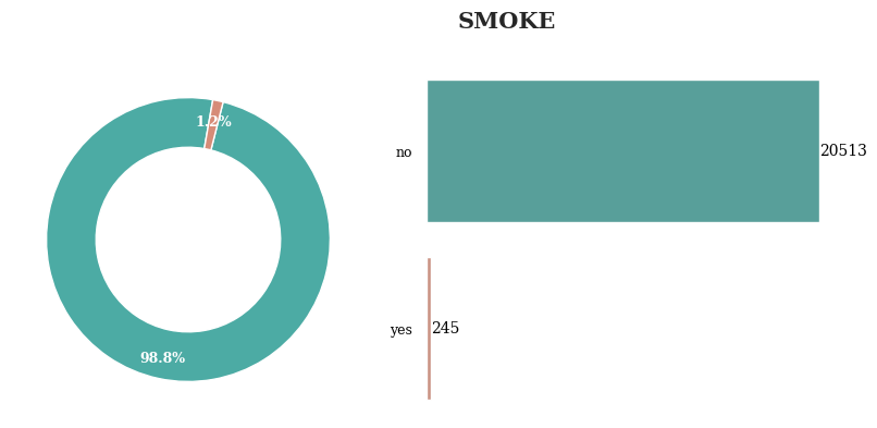
대부분의 경우 흡연을 하지 않음
따라서 특별하게 의미있다고 할 수 없음

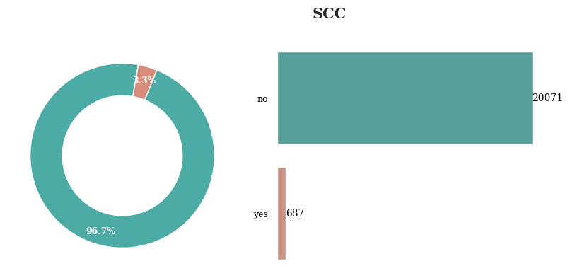
칼로리 소비 모니터링은 대부분의 경우 하지 않음
따라서 특별하게 의미있다고 할 수 없음

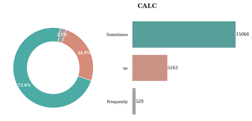
알코올 섭취 빈도는 Sometimes가 가장 높게 나타남

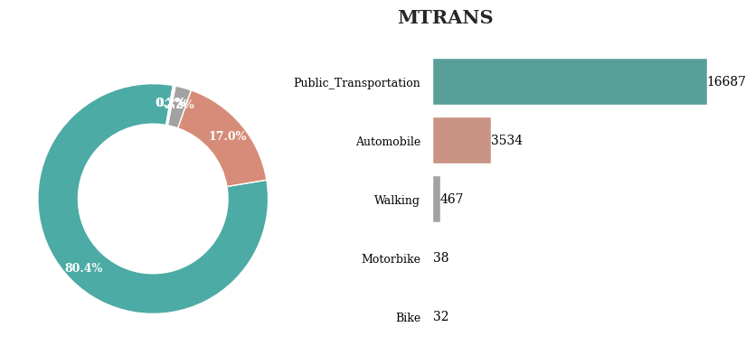
주로 이용하는 교통 수단은 대부분 Public_Transportation으로 나타남
약 97%의 사람들이 자동화 된 교통 수단을 이용하고 있고
약 2%의 사람들만이 직접 움직이는 방법을 사용하고 있음

Feature Engineering

결측치가 없는 관계로 결측치 대체는 따로 진행하지 않음

첫 번째 시도

각 feature에 대해 적절한 기준을 정의하고 그에 따라 값을 변환

Age

AgeGroup이라는 새로운 feature 정의

Height & Weight

BMI를 계산 후 새로운 feature 정의

no~Always로 나타난 feature

0~3으로 Encoding

yes or no로 나타난 feature

yes는 1, no는 0으로 Encoding

NCP

BMI에 따른 식사 빈도 계산

CH2O

Weight에 따른 수분 섭취량 계산

Gender

Male은 0, Female은 1로 Encoding

코드

def feature_engineering(df):
    # Age를 그룹화
    age_bins = [0, 18, 30, 40, 50, 80]
    df['AgeGroup'] = pd.cut(df['Age'], bins=age_bins, labels=False, right=False)

    # BMI 계산
    df['BMI'] = df['Weight'] / (df['Height'] ** 2)

    # 전자기기 사용 빈도 Encoding
    tech_bins = [0, 1, 2, 3]
    df['TechnologyUsageCategory'] = pd.cut(df['TUE'], bins=tech_bins, labels=False, right=False)

    # 활동 빈도 Encoding
    activity_bins = [0, 1, 2, np.inf]
    df['ActivityLevel'] = pd.cut(df['FAF'], bins=activity_bins, labels=['Low', 'Medium', 'High'], right=False)

    # BMI에 따른 식사 빈도 계산
    df['bmioncp'] = df['BMI'] / df['NCP']

    # 체중에 따른 수분 섭취 빈도 계산
    df['WIR'] = df['Weight'] / df['CH2O']

    # Gender Encoding
    df['Gender'] = df['Gender'].map({'Male':0, 'Female':1})

    # family_history_with_overweight Encoding
    df['family_history_with_overweight'] = df['family_history_with_overweight'].map({'no':0, 'yes':1})

    # FAVC Encoding
    df['FAVC'] = df['FAVC'].map({'no':0, 'yes':1})

    # CAEC Encoding
    df['CAEC'] = df['CAEC'].map({'no':0, 'Sometimes':1, 'Frequently':2, 'Always':3})

    # SMOKE Encoding
    df['SMOKE'] = df['SMOKE'].map({'no':0, 'yes':1})

    # SCC Encoding
    df['SCC'] = df['SCC'].map({'no':0, 'yes':1})

    # CALC 빈도 Encoding
    df['CALC'] = df['CALC'].map({'no':0, 'Sometimes':1, 'Frequently':2, 'Always':3})

    return df
    
train = feature_engineering(train)

test = feature_engineering(test)

두 번째 시도

첫 번째 방법과 다르게 복잡하게 생각하지 않고
새로 feature를 정의하지 않음

각 data type에 맞게 Encoding 진행

코드

# 범주형 데이터와 수치형 데이터를 구분 후 각각의 변수에 저장
# train과 test 두 데이터에 대해 각각 적용
num_cols = list(train.select_dtypes(exclude=['object']).columns)
cat_cols = list(train.select_dtypes(include=['object']).columns)

num_cols_test = list(test.select_dtypes(exclude=['object']).columns)
cat_cols_test = list(test.select_dtypes(include=['object']).columns)

# test의 경우 id는 제외하고 저장함
num_cols_test = [col for col in num_cols_test if col not in ['id']]

# StandardScaler를 통해 수치형 데이터를 표준화
scaler = StandardScaler()
train[num_cols] = scaler.fit_transform(train[num_cols])
test[num_cols_test] = scaler.transform(test[num_cols_test])

# LabelEncoder를 통해 범주형 데이터를 정수형으로 인코딩
labelencoder = LabelEncoder()
object_columns = train.select_dtypes(include='object').columns.difference(['NObeyesdad'])

# train 인코딩
for col_name in object_columns:
    if train[col_name].dtypes=='object':
        train[col_name]=labelencoder.fit_transform(train[col_name])

# test 인코딩
for col_name in test.columns:
    if test[col_name].dtypes=='object':
        test[col_name]=labelencoder.fit_transform(test[col_name])

Model Building

CatBoost / LGBM
두 모델 사용

공통적으로 최적 파라미터를 탐색(Grid Search)하고 최적 파라미터를 통해 결과물 출력

첫 번째 결과

CatBoost

LGBM

두 번째 결과

CatBoost

LGBM

두 번째 LGBM의 경우 Kaggle에 공개된 다른 코드를 통해 추가적인 방법 사용

Optuna 패키지를 통해 클래스별 임계값을 최적화
최적 임계값을 도출
.predict_proba를 통해 예측 확률 초기화
초기화 된 예측 확률과 최적 임계값을 통해 예측 확률을 예측값으로 변환

# Optuna를 통해 클래스별 임계값을 최적화

# objective 함수는 입력값의 임계값을 추출하고 thresholds 딕셔너리에 추가
def objective(trial):
    # Define the thresholds for each class
    thresholds = {}
    for i in range(num_classes):
        thresholds[f'threshold_{i}'] = trial.suggest_uniform(f'threshold_{i}', 0.0, 1.0)

    # apply_thresholds에서 변환된 값을 y_pred에 초기화
    y_pred = apply_thresholds(pred_proba, thresholds)

    # y_valid와 y_pred를 통해 accuracy score 계산
    accuracy = accuracy_score(y_valid, y_pred)
    
    return accuracy  

# apply_thresholds 함수는 입력된 임계값을 통해 확률을 예측 레이블로 변환
def apply_thresholds(y_proba, thresholds):
    y_pred_labels = np.argmax(y_proba, axis=1)
    for i in range(y_proba.shape[1]):
        y_pred_labels[y_proba[:, i] > thresholds[f'threshold_{i}']] = i

    return y_pred_labels

# num_classes 정의(best_param에 따름)
num_classes = 7

# Optuna의 Study 객체를 생성
study = optuna.create_study(direction='maximize')

# Objective 함수를 최적화
study.optimize(objective, n_trials=100)

# 최적 임계값을 초기화
best_thresholds = study.best_params

# 최적 임계값 출력
print("Best Thresholds:", best_thresholds)

# X_test에 대한 예측 확률을 test_label에 초기화
test_label = model_lgb.predict_proba(X_test)

# test_label에 초기화된 예측 확률을 apply_thresholds 함수를 통해 예측값으로 변환
test_label = apply_thresholds(test_label, best_thresholds)