안녕하세요. 밍기뉴와제제입니다.
이전에 제가 tensorflow2를 이용해 YOLOv1를 구현한 글을 작성한 적이 있습니다. 링크
이번에는 파이토치(PyTorch)로 YOLOv1를 구현해봤습니다. 정확히는 번역에 가깝습니다. 코드를 구현하며 느낀점은 파이토치가 더 편리하다는 것이었습니다. 데이터셋 전처리도 더 편하고, 학습도 더 편리하게 할 수 있더군요. 왜 시작을 텐서플로우로 해서...ㅠㅠ
그래도 덕분에 텐서플로우랑 파이토치로 짜여진 코드를 모두 이해할 수 있는 사람이 되어 뿌듯합니다. 홀홀.
그러면 지금부터 코드리뷰를 시작하겠습니다.
Import
import torch # 파이토치
import torch.nn as nn # 레이어, 활성화함수 등 basic building blocks이 들어있습니다.
import torchvision.transforms as transforms # 변환 연산(resize 등)이 들어있는 모듈입니다.
from torchvision.datasets import VOCDetection # PASCAL VOC 2007을 가져오는데 쓰입니다. 클래스 형식으로 만들어져 사용을 편리하게 할 수 있습니다.

import xmltodict # xml파일의 내용을 딕셔너리에 저장할 수 있는 메소드들이 들어있는 모듈입니다.
from PIL import Image # 이미지를 읽기 위해 사용합니다
import numpy as np # 넘파이, 저는 넘파이로 연산하는게 익숙해 넘파이를 사용합니다.
from tqdm import tqdm # tqdm, for문의 진행상황을 보기 위해 사용합니다.
먼저 모듈을 가져와야합니다. 파이토치는 텐서플로우와 달리 지원되는게 많습니다. 제일 큰 차이를 느꼈던게 데이터셋 전처리 부분이었는데요, 파이토치에서는 유명 데이터셋(PASCAL, COCO, MNIST 등)을 편리하게 사용할 수 있게 지원해줍니다.
데이터셋 전처리
파이토치는 데이터셋을 모델 학습에 편리하게 사용할 수 있는 DataLoader를 지원합니다. DataLoader는 dataset 클래스를 매개변수로 받아 생성되는 클래스인데요, dataset 클래스의 예로는 VOCDetection이 있습니다.
여기서 파이토치의 강점이 드러납니다. 파이토치는 데이터셋 클래스를 상속하여 나만의 데이터셋 클래스를 정의할 수 있는데요, 그 중 데이터셋에 있는 데이터쌍(x,y)를 인덱싱할 때 호출되는 getitem 함수에서 데이터 전처리를 수행할 수 있습니다.
class YOLO_PASCAL_VOC(VOCDetection):
    def __getitem__(self, index):
        img = (Image.open(self.images[index]).convert('RGB')).resize((224, 224))
        img_transform = transforms.Compose([transforms.PILToTensor(), transforms.Resize((224, 224))])
        img = torch.divide(img_transform(img), 255)


        target = xmltodict.parse(open(self.annotations[index]).read())

        classes = ["aeroplane", "bicycle", "bird", "boat", "bottle",
                   "bus", "car", "cat", "chair", "cow", "diningtable",
                   "dog", "horse", "motorbike", "person", "pottedplant",
                   "sheep", "sofa", "train", "tvmonitor"]

        label = np.zeros((7, 7, 25), dtype = float)

        Image_Height = float(target['annotation']['size']['height'])
        Image_Width  = float(target['annotation']['size']['width'])

        # 바운딩 박스 정보 받아오기
        try:
            for obj in target['annotation']['object']:

                # class의 index 휙득
                class_index = classes.index(obj['name'].lower())

                # min, max좌표 얻기
                x_min = float(obj['bndbox']['xmin'])
                y_min = float(obj['bndbox']['ymin'])
                x_max = float(obj['bndbox']['xmax'])
                y_max = float(obj['bndbox']['ymax'])

                # 224*224에 맞게 변형시켜줌
                x_min = float((224.0/Image_Width)*x_min)
                y_min = float((224.0/Image_Height)*y_min)
                x_max = float((224.0/Image_Width)*x_max)
                y_max = float((224.0/Image_Height)*y_max)

                # 변형시킨걸 x,y,w,h로 만들기
                x = (x_min + x_max)/2.0
                y = (y_min + y_max)/2.0
                w = x_max - x_min
                h = y_max - y_min

                # x,y가 속한 cell알아내기
                x_cell = int(x/32) # 0~6
                y_cell = int(y/32) # 0~6
                # cell의 중심 좌표는 (0.5, 0.5)다
                x_val_inCell = float((x - x_cell * 32.0)/32.0) # 0.0 ~ 1.0
                y_val_inCell = float((y - y_cell * 32.0)/32.0) # 0.0 ~ 1.0

                # w, h 를 0~1 사이의 값으로 만들기
                w = w / 224.0
                h = h / 224.0

                class_index_inCell = class_index + 5

                label[y_cell][x_cell][0] = x_val_inCell
                label[y_cell][x_cell][1] = y_val_inCell
                label[y_cell][x_cell][2] = w
                label[y_cell][x_cell][3] = h
                label[y_cell][x_cell][4] = 1.0
                label[y_cell][x_cell][class_index_inCell] = 1.0


        # single-object in image
        except TypeError as e :
            # class의 index 휙득
            class_index = classes.index(target['annotation']['object']['name'].lower())

            # min, max좌표 얻기
            x_min = float(target['annotation']['object']['bndbox']['xmin'])
            y_min = float(target['annotation']['object']['bndbox']['ymin'])
            x_max = float(target['annotation']['object']['bndbox']['xmax'])
            y_max = float(target['annotation']['object']['bndbox']['ymax'])

            # 224*224에 맞게 변형시켜줌
            x_min = float((224.0/Image_Width)*x_min)
            y_min = float((224.0/Image_Height)*y_min)
            x_max = float((224.0/Image_Width)*x_max)
            y_max = float((224.0/Image_Height)*y_max)

            # 변형시킨걸 x,y,w,h로 만들기
            x = (x_min + x_max)/2.0
            y = (y_min + y_max)/2.0
            w = x_max - x_min
            h = y_max - y_min

            # x,y가 속한 cell알아내기
            x_cell = int(x/32) # 0~6
            y_cell = int(y/32) # 0~6
            x_val_inCell = float((x - x_cell * 32.0)/32.0) # 0.0 ~ 1.0
            y_val_inCell = float((y - y_cell * 32.0)/32.0) # 0.0 ~ 1.0

            # w, h 를 0~1 사이의 값으로 만들기
            w = w / 224.0
            h = h / 224.0

            class_index_inCell = class_index + 5

            label[y_cell][x_cell][0] = x_val_inCell
            label[y_cell][x_cell][1] = y_val_inCell
            label[y_cell][x_cell][2] = w
            label[y_cell][x_cell][3] = h
            label[y_cell][x_cell][4] = 1.0
            label[y_cell][x_cell][class_index_inCell] = 1.0

        return img, torch.tensor(label)
이렇게 말이죠. 원래 입력 이미지의 사이즈도 제각각이도 라벨 데이터도 YOLO에 사용할 수 있는 방식이 아니었는데 getitem에서 전처리 코드를 넣음으로써 데이터셋에서 데이터를 꺼낼 때 전처리된 데이터를 얻을 수 있게 되었습니다.
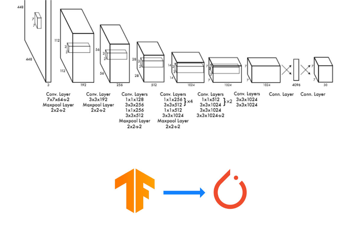
모델 설계
모델 설계 코드 역시 심플해졌습니다. 초기화(init), 정전파(forward)만 구현하면 끝이었고 메소드를 구현한 함수들 역시 심플했습니다.
class YOLO(torch.nn.Module):
    def __init__(self, VGG16):
        super(YOLO, self).__init__()
        self.backbone = VGG16

        self.conv = nn.Sequential(
            nn.Conv2d(in_channels = 512,out_channels = 1024, kernel_size = 3, padding = 1),
            nn.LeakyReLU(),
            nn.Conv2d(in_channels = 1024,out_channels = 1024, kernel_size = 3, padding = 1),
            nn.LeakyReLU(),
            nn.MaxPool2d(2),
            nn.Conv2d(in_channels = 1024,out_channels = 1024, kernel_size = 3, padding = 1),
            nn.LeakyReLU(),
            nn.Conv2d(in_channels = 1024,out_channels = 1024, kernel_size = 3, padding = 1),
            nn.LeakyReLU(),
            nn.Flatten()
        )
        self.linear = nn.Sequential(
            nn.Linear(7*7*1024, 4096),
            nn.LeakyReLU(),
            nn.Dropout(),
            nn.Linear(4096, 1470)
        )

        # 가중치 초기화
        for m in self.conv.modules():
    	    if isinstance(m, nn.Conv2d) :
		        nn.init.normal_(m.weight, mean=0, std=0.01)

        for m in self.linear.modules():
        	if isinstance(m, nn.Linear) :
                 nn.init.normal_(m.weight, mean=0, std=0.01)


    # 정전파
    def forward(self, x):
        out = self.backbone(x)
        out = self.conv(out)
        out = self.linear(out)
        out = torch.reshape(out, (-1 ,7, 7, 30))
        return out
코드만 봐도 연산이 어떻게 될지 그려집니다. 한가지 아쉬운 점은 레이어(conv2d, linear)를 추가할 때 가중치 초기화 방식을 선택할 수 없고 메서드를 호출해 따로 초기화를 해야하는 점이었습니다.
loss 함수
def yolo_multitask_loss(y_pred, y_true): # 커스텀 손실함수. 배치 단위로 값이 들어온다

    batch_loss = 0
    count = len(y_true)
    for i in range(0, len(y_true)) :
        y_true_unit = y_true[i].clone().detach().requires_grad_(True)

        y_pred_unit = y_pred[i].clone().detach().requires_grad_(True)

        y_true_unit = torch.reshape(y_true_unit, [49, 25])
        y_pred_unit = torch.reshape(y_pred_unit, [49, 30])

        loss = 0

        for j in range(0, len(y_true_unit)) :
            # pred = [1, 30], true = [1, 25]

            bbox1_pred = y_pred_unit[j, :4].clone().detach().requires_grad_(True)
            bbox1_pred_confidence = y_pred_unit[j, 4].clone().detach().requires_grad_(True)
            bbox2_pred = y_pred_unit[j, 5:9].clone().detach().requires_grad_(True)
            bbox2_pred_confidence = y_pred_unit[j, 9].clone().detach().requires_grad_(True)
            class_pred = y_pred_unit[j, 10:].clone().detach().requires_grad_(True)

            bbox_true = y_true_unit[j, :4].clone().detach().requires_grad_(True)
            bbox_true_confidence = y_true_unit[j, 4].clone().detach().requires_grad_(True)
            class_true = y_true_unit[j, 5:].clone().detach().requires_grad_(True)

            # IoU 구하기
            # x,y,w,h -> min_x, min_y, max_x, max_y로 변환
            box_pred_1_np = bbox1_pred.detach().numpy()
            box_pred_2_np = bbox2_pred.detach().numpy()
            box_true_np   = bbox_true.detach().numpy()

            box_pred_1_area = box_pred_1_np[2] * box_pred_1_np[3]
            box_pred_2_area = box_pred_2_np[2] * box_pred_2_np[3]
            box_true_area   = box_true_np[2]  * box_true_np[3]

            box_pred_1_minmax = np.asarray([box_pred_1_np[0] - 0.5*box_pred_1_np[2], box_pred_1_np[1] - 0.5*box_pred_1_np[3], box_pred_1_np[0] + 0.5*box_pred_1_np[2], box_pred_1_np[1] + 0.5*box_pred_1_np[3]])
            box_pred_2_minmax = np.asarray([box_pred_2_np[0] - 0.5*box_pred_2_np[2], box_pred_2_np[1] - 0.5*box_pred_2_np[3], box_pred_2_np[0] + 0.5*box_pred_2_np[2], box_pred_2_np[1] + 0.5*box_pred_2_np[3]])
            box_true_minmax   = np.asarray([box_true_np[0] - 0.5*box_true_np[2], box_true_np[1] - 0.5*box_true_np[3], box_true_np[0] + 0.5*box_true_np[2], box_true_np[1] + 0.5*box_true_np[3]])

            # 곂치는 영역의 (min_x, min_y, max_x, max_y)
            InterSection_pred_1_with_true = [max(box_pred_1_minmax[0], box_true_minmax[0]), max(box_pred_1_minmax[1], box_true_minmax[1]), min(box_pred_1_minmax[2], box_true_minmax[2]), min(box_pred_1_minmax[3], box_true_minmax[3])]
            InterSection_pred_2_with_true = [max(box_pred_2_minmax[0], box_true_minmax[0]), max(box_pred_2_minmax[1], box_true_minmax[1]), min(box_pred_2_minmax[2], box_true_minmax[2]), min(box_pred_2_minmax[3], box_true_minmax[3])]

            # 박스별로 IoU를 구한다
            IntersectionArea_pred_1_true = 0

            # 음수 * 음수 = 양수일 수도 있으니 검사를 한다.
            if (InterSection_pred_1_with_true[2] - InterSection_pred_1_with_true[0] + 1) >= 0 and (InterSection_pred_1_with_true[3] - InterSection_pred_1_with_true[1] + 1) >= 0 :
                    IntersectionArea_pred_1_true = (InterSection_pred_1_with_true[2] - InterSection_pred_1_with_true[0] + 1) * InterSection_pred_1_with_true[3] - InterSection_pred_1_with_true[1] + 1

            IntersectionArea_pred_2_true = 0

            if (InterSection_pred_2_with_true[2] - InterSection_pred_2_with_true[0] + 1) >= 0 and (InterSection_pred_2_with_true[3] - InterSection_pred_2_with_true[1] + 1) >= 0 :
                    IntersectionArea_pred_2_true = (InterSection_pred_2_with_true[2] - InterSection_pred_2_with_true[0] + 1) * InterSection_pred_2_with_true[3] - InterSection_pred_2_with_true[1] + 1

            Union_pred_1_true = box_pred_1_area + box_true_area - IntersectionArea_pred_1_true
            Union_pred_2_true = box_pred_2_area + box_true_area - IntersectionArea_pred_2_true

            IoU_box_1 = IntersectionArea_pred_1_true/Union_pred_1_true
            IoU_box_2 = IntersectionArea_pred_2_true/Union_pred_2_true

            responsible_box = 0
            responsible_bbox_confidence = 0
            non_responsible_bbox_confidence = 0

            # box1, box2 중 responsible한걸 선택(IoU 기준)
            if IoU_box_1 >= IoU_box_2 :
                responsible_box = bbox1_pred.clone().detach().requires_grad_(True)
                responsible_bbox_confidence = bbox1_pred_confidence.clone().detach().requires_grad_(True)
                non_responsible_bbox_confidence = bbox2_pred_confidence.clone().detach().requires_grad_(True)

            else :
                responsible_box = bbox2_pred.clone().detach().requires_grad_(True)
                responsible_bbox_confidence = bbox2_pred_confidence.clone().detach().requires_grad_(True)
                non_responsible_bbox_confidence = bbox1_pred_confidence.clone().detach().requires_grad_(True)

            # 1obj(i) 정하기(해당 셀에 객체의 중심좌표가 들어있는가?)
            obj_exist = torch.ones_like(bbox_true_confidence)
            if box_true_np[0] == 0.0 and box_true_np[1] == 0.0 and box_true_np[2] == 0.0 and box_true_np[3] == 0.0 :
                obj_exist = torch.zeros_like(bbox_true_confidence)


            # 만약 해당 cell에 객체가 없으면 confidence error의 no object 파트만 판단. (label된 값에서 알아서 해결)
            # 0~3 : bbox1의 위치 정보, 4 : bbox1의 bbox confidence score, 5~8 : bbox2의 위치 정보, 9 : bbox2의 confidence score, 10~29 : cell에 존재하는 클래스 확률 = pr(class | object)

            # localization error 구하기(x,y,w,h). x, y는 해당 grid cell의 중심 좌표와 offset이고 w, h는 전체 이미지에 대해 정규화된 값이다. 즉, 범위가 0~1이다.
            localization_err_x = torch.pow( torch.subtract(bbox_true[0], responsible_box[0]), 2) # (x-x_hat)^2
            localization_err_y = torch.pow( torch.subtract(bbox_true[1], responsible_box[1]), 2) # (y-y_hat)^2

            localization_err_w = torch.pow( torch.subtract(torch.sqrt(bbox_true[2]), torch.sqrt(responsible_box[2])), 2) # (sqrt(w) - sqrt(w_hat))^2
            localization_err_h = torch.pow( torch.subtract(torch.sqrt(bbox_true[3]), torch.sqrt(responsible_box[3])), 2) # (sqrt(h) - sqrt(h_hat))^2

            # nan 방지
            if torch.isnan(localization_err_w).detach().numpy() == True :
                localization_err_w = torch.zeros_like(localization_err_w)

            if torch.isnan(localization_err_h).detach().numpy() == True :
                localization_err_h = torch.zeros_like(localization_err_h)

            localization_err_1 = torch.add(localization_err_x, localization_err_y)
            localization_err_2 = torch.add(localization_err_w, localization_err_h)
            localization_err = torch.add(localization_err_1, localization_err_2)

            weighted_localization_err = torch.multiply(localization_err, 5.0) # 5.0 : λ_coord
            weighted_localization_err = torch.multiply(weighted_localization_err, obj_exist) # 1obj(i) 곱하기

            # confidence error 구하기. true의 경우 답인 객체는 1 * ()고 아니면 0*()가 된다.
            # index 4, 9에 있는 값(0~1)이 해당 박스에 객체가 있을 확률을 나타낸거다. Pr(obj in bbox)

            class_confidence_score_obj = torch.pow(torch.subtract(responsible_bbox_confidence, bbox_true_confidence), 2)
            class_confidence_score_noobj = torch.pow(torch.subtract(non_responsible_bbox_confidence, torch.zeros_like(bbox_true_confidence)), 2)
            class_confidence_score_noobj = torch.multiply(class_confidence_score_noobj, 0.5)

            class_confidence_score_obj = torch.mul(class_confidence_score_obj, obj_exist)
            class_confidence_score_noobj = torch.mul(class_confidence_score_noobj, torch.subtract(torch.ones_like(obj_exist), obj_exist)) # 객체가 존재하면 0, 존재하지 않으면 1을 곱합

            class_confidence_score = torch.add(class_confidence_score_obj,  class_confidence_score_noobj)

            # classification loss(10~29. 인덱스 10~29에 해당되는 값은 Pr(Class_i|Object)이다. 객체가 cell안에 있을 때 해당 객체일 확률
            # class_true_oneCell는 진짜 객체의 인덱스에 해당하ㄴ 원소의 값만 1이고 나머지는 0

            torch.pow(torch.subtract(class_true, class_pred), 2.0) # 여기서 에러

            classification_err = torch.pow(torch.subtract(class_true, class_pred), 2.0)
            classification_err = torch.sum(classification_err)
            classification_err = torch.multiply(classification_err, obj_exist)

            # loss합체
            loss_OneCell_1 = torch.add(weighted_localization_err, class_confidence_score)

            loss_OneCell = torch.add(loss_OneCell_1, classification_err)

            if loss == 0 :
                loss = loss_OneCell.clone().detach().requires_grad_(True)
            else :
                loss = torch.add(loss, loss_OneCell)

        if batch_loss == 0 :
            batch_loss = loss.clone().detach().requires_grad_(True)
        else :
            batch_loss = torch.add(batch_loss, loss)

    # 배치에 대한 loss 구하기
    batch_loss = torch.divide(batch_loss, count)

    return batch_loss
깁니다. 많이 깁니다. Loss함수를 다시 작성하며 파이토치에서 지원하는 텐서간 연산 함수의 사용법을 많이 익힐 수 있었습니다.
Train 함수
def train_YOLO(YOLO_model, criterion, optimizer, epochs, data_loader, device) :
    # 학습 -> 성능 측정

    pbar = tqdm(range(epochs), desc="training", mininterval=0.01)

    for epoch in pbar:  # loop over the dataset multiple times
        optimizer.param_groups[0]['lr']
        if epoch >=0 and epoch < 75 :
            optimizer.param_groups[0]['lr'] = 0.001 + 0.009 * (float(epoch)/(75.0)) # 가중치를 0.001 ~ 0.01로 변경
        elif epoch >= 75 and epoch < 105 :
            optimizer.param_groups[0]['lr'] = 0.001
        else :
            optimizer.param_groups[0]['lr'] = 0.0001

        for inputs, labels in data_loader:

            # 데이터 꺼내기(배치 단위)
            inputs = inputs.to(device)
            labels = labels.to(device)

            optimizer.zero_grad() # 그레디언트 초기화

            outputs = YOLO_model(inputs) # 예측값 휙득
            loss = criterion(outputs, labels) # loss 휙득
            loss.backward() # 그레디언트 구하기
            optimizer.step() # 구한 그레이던트를 이용해 가중치 업데이트

            # 배치로 학습시킬 때마다 loss 보여주기
            pbar_str = "training, [loss = %.4f]" % loss.item()
            pbar.set_description(pbar_str)

    return YOLO_model
텐서플로우와 많은 차이점을 느낀 또다른 부분이 바로 모델 학습이었습니다.
텐서플로우는 loss와 optimizer를 정한 뒤 학습을
optimizer = tf.keras.optimizers.SGD(learning_rate=0.001, momentum = 0.9)

YOLO.compile(loss = yolo_multitask_loss, optimizer=optimizer, run_eagerly=True)

YOLO.fit(train_image_dataset, train_label_dataset,
          batch_size=BATCH_SIZE,
          validation_data = (val_image_dataset, val_label_dataset),
          epochs=EPOCH,
          verbose=1,
          callbacks=[checkpoint, tf.keras.callbacks.LearningRateScheduler(lr_schedule)])
이렇게 모델 클래스 내 메소드인 fit()을 호출하면 알아서 학습이 되었는데 파이토치는 fit()에 해당하는 학습 함수를 직접 구현하였습니다.
허나 학습 함수를 직접 구현하는 것이 저한테 더 맞았습니다. fit()에서 에러가 발생하면 뭐가 문제인지 디버깅 하는게 어려웠는데 제가 제가 직접 만든 학습 함수는 코드를 하나씩 다 확인하며 디버깅을 할 수 있기 때문입니다. 학습 함수를 구현하는게 쉽기 때문에 더 마음에 든게 아닌가 싶기도 하네요.
돌려보기
이제 작성한 함수, 클래스를 이용해 모델 학습을 시켜봅시다. 아래의 코드로 모델 생성 + 학습을 구현할 수 있습니다.
device = 'cuda' if torch.cuda.is_available() else 'cpu' # gpu를 사용할지 cpu를 사용할지 결정합니다.

# VOC 2007 dataset의 위치를 저장합니다.
current_path = os.getcwd()
path2data = current_path + '/voc'
if not os.path.exists(path2data): # 만약 데이터셋이 저장되어 있지 않다면
    os.mkdir(path2data) # 저장할 폴더를 생성합니다.

BATCH_SIZE = 64
EPOCH = 135

# 데이터셋을 편하게 사용할 수 있는 데이터셋 클래스의 객체를 선언합니다.
# 만약 데이터셋이 없으면 해당 데이터셋이 있을 경로(path2data)에 데이터셋을 다운로드합니다.
Train_Dataset = YOLO_PASCAL_VOC(path2data, year='2007', image_set='train', download=True)
Test_Dataset = YOLO_PASCAL_VOC(path2data, year='2007', image_set='test', download=True)

# 생성한 데이터셋 객체로 DataLoader 객체를 생성합니다.
# DataLoader를 이용하면 미니배치 단위로 모델에 데이터를 넣는 것이 매우 쉬워집니다.
# 즉, 학습시키는 코드를 쉽게 구현할 수 있게 해줍니다.
data_loader = torch.utils.data.DataLoader(dataset=Train_Dataset, # 사용할 데이터셋
                                          batch_size=BATCH_SIZE, # 미니배치 크기
                                          shuffle=True, # 에포크마다 데이터셋 셔플할건가?
                                          drop_last=True) # 마지막 배치가 BATCH_SIZE보다 작을 때, 마지막 배치를 사용하지 않으려면 True를, 사용할거면 False를 입력합니다.

# 사전학습된 VGG16을 불러옵니다.
VGGNet = torch.hub.load('pytorch/vision:v0.10.0', 'vgg16', pretrained=True)
# VGG16에 있는 레이어 중 제가 사용할 레이어들이 그레디언트 추적을 못하게 해 가중치 변화를 막고
# padding을 1로 만들어 same padding이 되게끔 만들어줍니다.
for i in range(len(VGGNet.features[:-1])) :
    if type(VGGNet.features[i]) == type(nn.Conv2d(64,64,3)) :
        VGGNet.features[i].weight.requires_grad = False
        VGGNet.features[i].bias.requires_grad = False
        VGGNet.features[i].padding = 1

# YOLO와 optimizer를 선언합니다. VGGNet.features[:-1]는 VGG16에서 제가 Backbone으로 사용할 레이어들을 말합니다.
YOLO_model =  YOLO(VGGNet.features[:-1]).to(device) # Create YOLO model
optimizer = torch.optim.SGD(YOLO_model.parameters(), lr = 0.01, momentum = 0.9, weight_decay=0.0005)

# 모델을 학습시킵니다.
YOLO_model = train_YOLO(YOLO_model, yolo_multitask_loss, optimizer, EPOCH, data_loader, device)
코드를 읽으시다보면 어떤 흐름으로 모델을 생성하고 학습을 시킬 수 있는지 확인할 수 있습니다.
학습이 진행되는가?
학습이 진행되는지 제 노트북에서 돌려봤습니다.
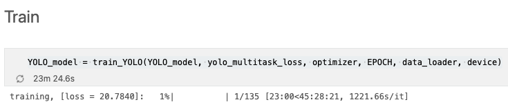
노트북이라 느리긴 하지만 학습이 된다는 사실을 확인할 수 있었습니다. 아마 cuda를 지원하는 gpu에서 돌리면 빠른 속도로 학습이 될 것으로 보입니다.
구현 후기
텐서플로우로 구현했던걸 파이토치로 재구현해서 그런지 오랜 시간이 걸리지 않았습니다. 비유하자면 표준어와 사투리의 차이? 정도로 느껴졌습니다.
그러니 파이토치 혹은 텐서플로우를 먼저 공부하신 분들도 서로 다른 프레임워크로 짜여졌다고 해서 코드 해석을 포기하지 마시고 차근차근 해석을 시도해보시길 바랍니다. 본인이 쓰던 프레임워크와 별다른 차이가 없음을 금방 깨달을실 겁니다.
원래 이번글은 논문 리뷰를 하려고 했는데 파이토치 코드 구현글을 쓰게 되었네요. 다음글로 무엇을 쓸지 저도 궁금해집니다.
그러면 다음글에서 뵙겠습니다.