
10. 다양한 데이터 전처리 기법
10-1. 들어가며
학습목표
- 중복된 데이터를 찾아 제거, 결측치(missing data)를 제거하거나 채워 넣기
- 데이터를 정규화
- 이상치(outlier)를 찾고, 이를 처리
- 범주형 데이터를 원-핫 인코딩
- 연속적인 데이터를 구간으로 나눠 범주형 데이터로 변환
데이터를 준비하기
trade.csv - 관세청 수출입 무역 통계 에서 가공한 데이터
-
클라우드에 연걸
$ mkdir -p ~/aiffel/data_preprocess/ $ ln -s ~/data/ ~/aiffel/data_preprocess/ -
데이터 불러오기
import pandas as pd
import numpy as np
import matplotlib.pyplot as plt
import os

csv_file_path = os.getenv('HOME')+'/aiffel/data_preprocess/data/trade.csv'
trade = pd.read_csv(csv_file_path)
trade.head()

<실행결과>
데이터프레임 출력
10-2. 결측치(Missing Data)
1. 결측치를 처리하는 방법
1) 결측치가 있는 데이터를 제거
2) 결측치를 어떤 값으로 대체
📌 데이터마다 특성을 반영하여 해결
2. 준비한 데이터의 결측치 여부 확인
1) 전체 데이터 건수 확인
print('전체 데이터 건수:', len(trade))

<실행결과>
전체 데이터 건수: 199
2) 전체 데이터 건수- Null 값이 아닌 행 개수 == 컬럼별 결측치의 개수
DataFrame.count() - 결측치가 있는 행 더해서 출력
print('컬럼별 결측치 개수')
len(trade) - trade.count()

<실행결과>
컬럼별 결측치 개수
기간        0
국가명       0
수출건수      3
수출금액      4
수입건수      3
수입금액      3
무역수지      4
기타사항    199
dtype: int64
3) 기타사항 행 삭제(전체 행이 결측치)
trade = trade.drop('기타사항', axis=1)
trade.head()
4) 결측치가 있는 행 찾기
DataFrame.isnull(): 데이터마다 결측치 여부를 True, False로 반환trade.isnull()
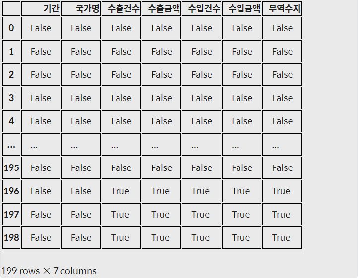
DataFrame.any(axis=1): 행마다 하나라도 True가 있으면 True, 그렇지 않으면 False를 반환trade.isnull().any(axis=1) <실행결과> 0 False 1 False 2 False 3 False 4 False ... 194 False 195 False 196 True 197 True 198 True Length: 199, dtype: bool- Dataframe.isnull().any(axis=1) : True인 데이터만 추출
trade[trade.isnull().any(axis=1)]
- DataFrame.dropna() : 결측치를 삭제해 주는 메서드
-
‘how’
- all : 모든 컬럼이 결측치 일 때 행 제거
- any : 컬럼 한 개라도 결측치일 때 행 제거
-
subset : 특정 컬럼들을 선택
-
inplace : DataFrame 내부에 바로 적용
trade.dropna(how='all', subset=['수출건수', '수출금액', '수입건수', '수입금액', '무역수지'], inplace=True)📌 어차피 행을 삭제할 거 라면 DataFrame. drop(제거할 행 인덱스)- 변수 재활당 필요, 여러 개라면 리스트로 전달
-
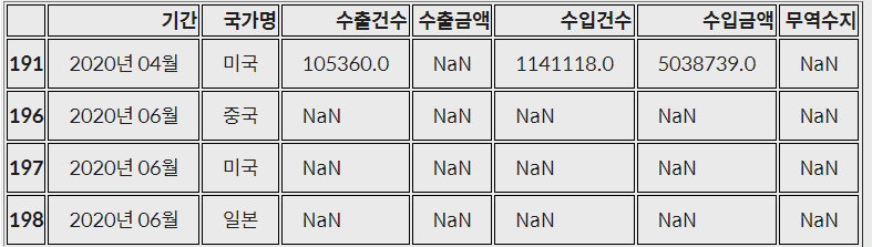
- 남아 있는 결측치 확인하기
trade[trade.isnull().any(axis=1)]
- 데이터를 보완하는 방법
- 평균, 중앙값 등으로 대체
- 시계열 특성을 가진 데이터의 경우 앞뒤 데이터를 통해 결측치를 대체
- 남은 결측치 보완하기 - 앞뒤 데이터를 이용해 결측치 대체
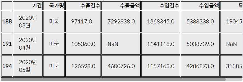
DataFrame.loc[행 라벨, 열 라벨]을 입력하면 해당 라벨을 가진 데이터를 출력**trade.loc[[188, 191, 194]]**
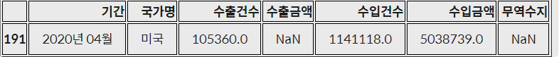
- index 191의 수출금액 컬럼값을 이전 달과 다음 달의 평균으로 채우기
trade.loc[191, '수출금액'] = (trade.loc[188, '수출금액'] + trade.loc[194, '수출금액'] )/2
trade.loc[[191]]
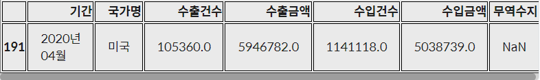
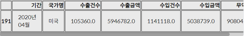
- index 191의 무역수지 컬럼은 수출금액과 수입금액의 차이를 이용하여 채우기
trade.loc[191, '무역수지'] = trade.loc[191, '수출금액'] - trade.loc[191, '수입금액']
trade.loc[[191]]
3. 범주형 데이터 결측치 처리
1. 특정 값을 지정해 줄 수 있습니다. 예를 들어 ‘기타’, ‘결측’과 같이 새로운 범주를 만들어 결측치를 채울 수 있습니다.
2. 최빈값 등으로 대체, 결측치가 많을 때는 다른 방법을 사용
3. 다른 데이터를 이용해 예측값으로 대체
4. 시계열 특성을 가진 데이터의 경우 앞뒤 데이터를 통해 결측치를 대체
- 특정인의 2019년 직업이 결측치이고, 2018년과 2020년 직업이 일치한다면 그 값으로 보완
- 다르다면 둘 중 하나로 보완
10-3. 중복된 데이터
1. 중복 데이터 확인
DataFrame.duplicated(): 중복된 데이터 여부를 불리언 값으로 반환trade.duplicated() <실행결과> 0 False 1 False 2 False 3 False 4 False ... 191 False 192 False 193 False 194 False 195 False Length: 196, dtype: bool- 중복된 행 추출
trade[trade.duplicated()]
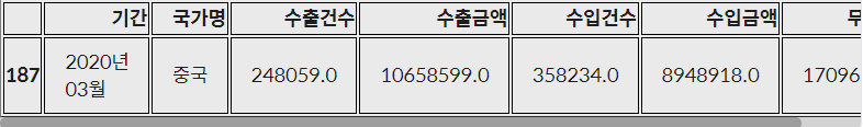
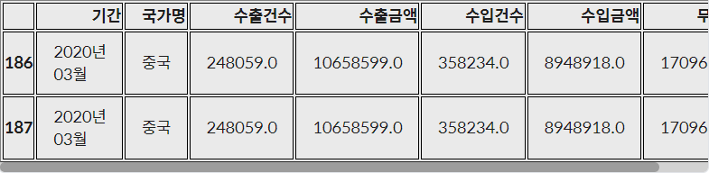
- 중복데이터 확인하기
```python
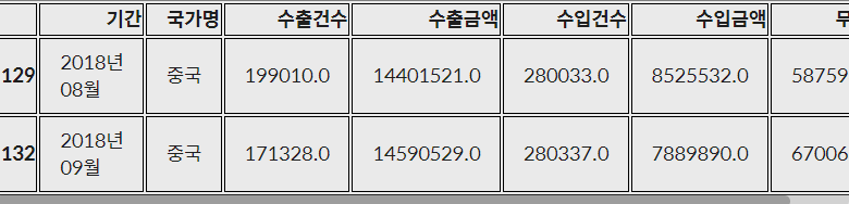
trade[(trade['기간']=='2020년 03월')&(trade['국가명']=='중국')]
```
DataFrame.drop_duplicates: 중복된 데이터 삭제-
subset = [중복된 컬럼]
-
keep = ‘last’ : 뒤에 있는 데이터 남기기
trade.drop_duplicates(inplace=True)
-
10-4. 이상치(Outlier)
이상치 제거하기
- 이상치를 삭제, 이상치를 원래 데이터에서 삭제하고, 이상치끼리 따로 분석
- 이상치를 다른 값으로 대체. 데이터가 적으면 다른 값으로 대체, 최댓값, 최솟값을 설정해 데이터의 범위를 제한 가능
- 다른 데이터를 활용하여 예측 모델을 만들어 예측값을 활용
- 아니면 binning을 통해 수치형 데이터를 범주형으로 바꾸기 가능
z-score method

outlier함수를 만들기- 이상치인 데이터의 인덱스를 리턴
- input : 데이터프레임
df, 컬럼col, 기준z abs(df[col] - np.mean(df[col])): 데이터에서 평균을 빼준 것에 절대값 구하기abs(df[col] - np.mean(df[col]))/np.std(df[col]): 위에 한 작업에 표준편차로 나눠주기df[abs(df[col] - np.mean(df[col]))/np.std(df[col])>z].index: 값이 z보다 큰 데이터의 인덱스를 추출
def outlier(df, col, z):
return df[abs(df[col] - np.mean(df[col]))/np.std(df[col])>z].index- 함수에 넣어서 추출한 인덱스를 이용해 DataFrame 출력하기 - z = 1.5
trade.loc[outlier(trade, '무역수지', 1.5)]
- 함수에 넣어서 추출한 인덱스를 이용해 DataFrame 출력하기 - z = 2
trade.loc[outlier(trade, '무역수지', 2)]
not_outlier(): 무역수지가 이상치 값이 아닌 데이터만 추출하는 함수def not_outlier(df, col, z): return df[abs(df[col] - np.mean(df[col]))/np.std(df[col]) <= z].index
IQR method - 사분위 수를 이용한 이상치 제거
- 사분위 범위수 IQR(Interquartile range)을 이용
- 이상치
- Q1−1.5∗IQR 보다 왼쪽에 있거나 Q_3 + 1.5IQRQ3+1.5∗IQR*보다 오른쪽에 있는 경우
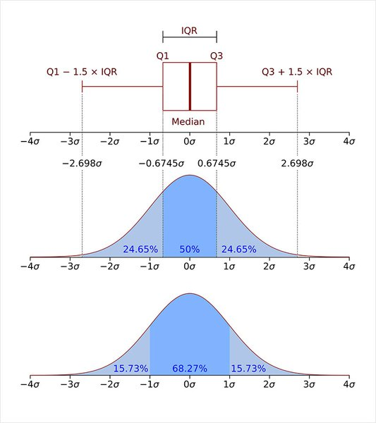
**[출처 : https://en.wikipedia.org/wiki/Interquartile_range]**- 제1사분위수와 제 3사분위수를 구하기 -
-
np.percentile() : 백분위수 구하는 함수
- 수의 범위 : 0 ~ 100Q3, Q1 = np.percentile(data, [75 ,25]) IQR = Q3 - Q1 IQR <실행결과> 1.1644925829790964
-
- IQR과 제 1사분위수, 제 3사분위수를 이용하여 이상치를 확인
data[(Q1-1.5*IQR > data)|(Q3+1.5*IQR < data)]

<실행결과>
array([ 2.31256634,  8.        , 10.        , -3.        , -5.        ])
z-score 방법이 가지는 단점
- 평균과 표준편차 자체가 이상치의 존재에 크게 영향을 받기 때문
- 작은 데이터셋의 경우 z-score의 방법으로 이상치를 알아내기 어렵다. 특히 item이 12개 이하인 데이터셋에서는 불가능
10-5. 정규화(Normalization)
정규화 방법
-
표준화(Standardization)
Standaridization 데이터의 평균은 0, 분산은 1로 변환 -
Min-Max Scaling
Min-Max Scaling 데이터의 최솟값은 0, 최댓값은 1로 변환
Standardization - trade DataFrame - 표준편차가 1로 변환
- 수치형 컬럼들을 cols 변수에 담은 후, 데이터에서 평균을 빼고, 표준편차로 나눠주기
# trade 데이터를 Standardization 기법으로 정규화합니다.
cols = ['수출건수', '수출금액', '수입건수', '수입금액', '무역수지']
trade_Standardization= (trade[cols]-trade[cols].mean())/trade[cols].std()
trade_Standardization.head()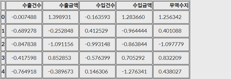
Min-Max Scaling - 최솟값 → 0, 최댓값 → 1로 변환
- 데이터에서 최솟값을 빼주고, '최댓값-최솟값'으로 나눠주기
# trade 데이터를 min-max scaling 기법으로 정규화합니다.
trade[cols] = (trade[cols]-trade[cols].min())/(trade[cols].max()-trade[cols].min())
trade.head()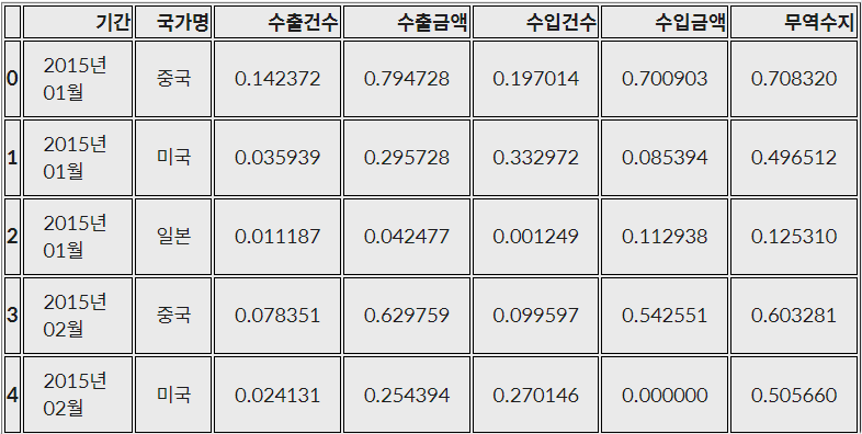
trade.describe()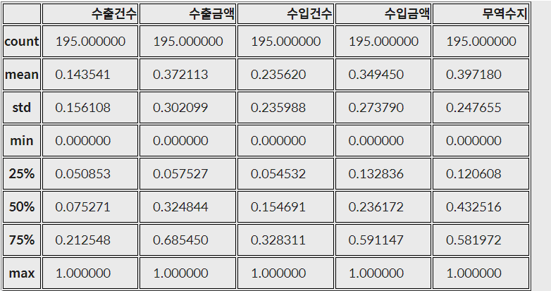
판다스 Min - Max scaling
- 판다스로 DataFrame 만들기
# 훈련, 테스트 세트 데이터프레임 만들기
train = pd.DataFrame([[10, -10], [30, 10], [50, 0]])
test = pd.DataFrame([[0, 1], [10, 10]])

train_min = train.min()
train_max = train.max()

train_min_max = (train - train_min)/(train_max - train_min)

# test를 min-max scaling할 때도 train 정규화 기준으로 수행
test_min_max =  (test - train_min)/(train_max - train_min)
train_min_max
test_min_max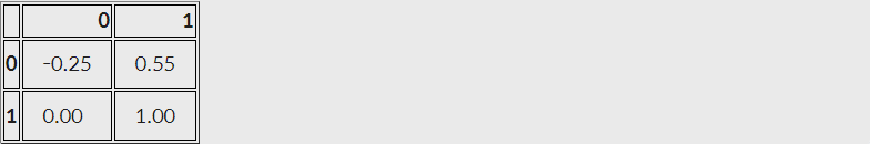
scikit-learn의 StandardScaler, MinMaxScaler를 사용
from sklearn.preprocessing import MinMaxScaler
train = [[10, -10], [30, 10], [50, 0]]
test = [[0, 1]]
scaler = MinMaxScaler()- train의 min, max출력
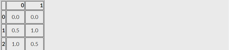
scaler.fit_transform(train)

실행결과
array([[0. , 0. ],
       [0.5, 1. ],
[1. , 0.5]])- test의 min, max출력
scaler.transform(test)

<실행결과>
array([[-0.25,  0.55]])
10-6. 원-핫 인코딩(One-Hot Encoding)
카테고리별 이진 특성을 만들어 해당하는 특성만 1, 나머지는 0으로 만드는 방법
pandas에서 get_dummies 함수를 통해 손쉽게 원-핫 인코딩
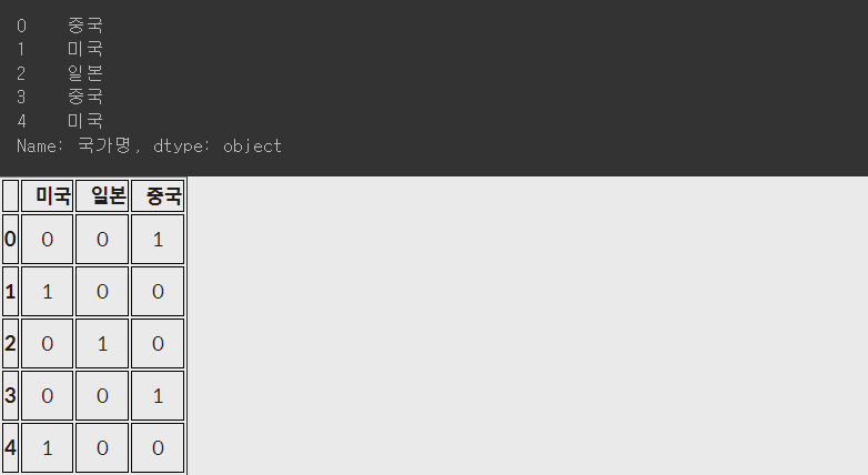
#trade 데이터의 국가명 컬럼 원본
print(trade['국가명'].head())

# get_dummies를 통해 국가명 원-핫 인코딩
country = pd.get_dummies(trade['국가명'])
country.head()

<실행결과>
pd.concat 함수로 데이터프레임 trade와 country를 합쳐주기
trade = pd.concat([trade, country], axis=1)
trade.head()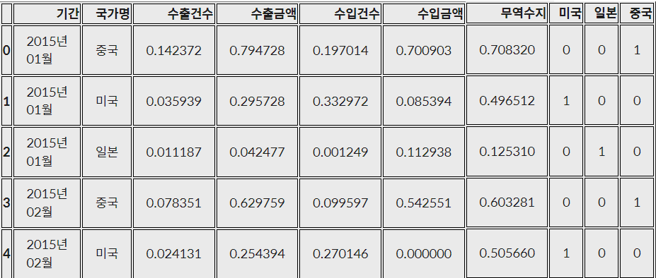
불필요한 행 삭제 - 완벽한 DataFrmae 완성
trade.drop(['국가명'], axis=1, inplace=True)
trade.head()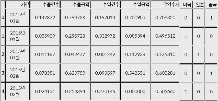
10-7. 구간화(Data Binning) or bucketing
구간화 : 수치형, 연속형 데이터를 범주형 데이터로 바꾸는 과정
- 연속적인 데이터를 구간을 나눠 분석
pd.cut()을 이용해 구간 나누기
- .cut(data, bins, right, labels)
- data : 구간을 나눌 데이터
- bins : 자료를 구분하는 구간
- 리스트 형태 : 리스트가에 있는 값들로 구분
- 정수 : 전체 구간을 정수로 개수만큼 구분
- right : 등호의 위치
- False(기본값) : 등호가 왼쪽에 위치
- True : 등호가 오른쪽에 위치
- labels : 구분한 범주의 라벨
import pandas as pd
import numpy as np

# 리스트를 판다스 시리즈로 만들기
salary = pd.Series([4300, 8370, 1750, 3830, 1840, 4220, 3020, 2290, 4740, 4600,
                    2860, 3400, 4800, 4470, 2440, 4530, 4850, 4850, 4760, 4500,
                    4640, 3000, 1880, 4880, 2240, 4750, 2750, 2810, 3100, 4290,
                    1540, 2870, 1780, 4670, 4150, 2010, 3580, 1610, 2930, 4300,
                    2740, 1680, 3490, 4350, 1680, 6420, 8740, 8980, 9080, 3990,
                    4960, 3700, 9600, 9330, 5600, 4100, 1770, 8280, 3120, 1950,
                    4210, 2020, 3820, 3170, 6330, 2570, 6940, 8610, 5060, 6370,
                    9080, 3760, 8060, 2500, 4660, 1770, 9220, 3380, 2490, 3450,
                    1960, 7210, 5810, 9450, 8910, 3470, 7350, 8410, 7520, 9610,
                    5150, 2630, 5610, 2750, 7050, 3350, 9450, 7140, 4170, 3090])

bins = [0, 2000, 4000, 6000, 8000, 10000]

# 범주를 구분하는 기준
ctg = pd.cut(salary, bins=bins)
ctg

<실행결과>
0      (4000, 6000]
1     (8000, 10000]
2         (0, 2000]
3      (2000, 4000]
4         (0, 2000]
          ...
95     (2000, 4000]
96    (8000, 10000]
97     (6000, 8000]
98     (4000, 6000]
99     (2000, 4000]
Length: 100, dtype: category
Categories (5, interval[int64, right]): [(0, 2000] < (2000, 4000] < (4000, 6000] < (6000, 8000] < (8000, 10000]]- .value.counts() : 구간별로 값이 몇 개가 있는 지 확인
-
어떤 컬럼/Series의 unique value들을 count해주는 함수
-
.sort_index() : 인덱스를 기준으로 정렬(오름차순)
ctg.value_counts().sort_index()

<실행결과>
(0, 2000]        12
(2000, 4000]     34
(4000, 6000]     29
(6000, 8000]      9
(8000, 10000]    16
dtype: int64
-
pd.qcut() - 동일한 갯수로 구간 나누기
- 매개변수는 .cut()와 동일