해당 게시물은 아래 원문을 참조하여 작성되었습니다.
출처: https://e-dorigatti.github.io/math/deep%20learning/2023/06/25/diffusion

Simplest Implementation of Diffusion Models

이 튜토리얼은 Ho 2020, Denoising Diffusion Probabilistic Models에 따라, 가장 단순한 파이토치 기반 Diffusion(이하 확산) 모델 구현을 보여줍니다.

생성 모델은 tractable(즉, 단순한) 분포를 따르는 잠재 변수에서 새로운 샘플(예: 이미지) 생성을 학습합니다. 최근 확산 모델은 강력하고 유능한 생성 모델의 일종으로 부상했으며, Stable Diffusion, Midjourney, DALL·E 등 최신 생성 AI 사례의 기반이 되고 있습니다. (23년 6월 기준)
확산 모델은 관심 있는 데이터 분포(이미지 등)에서 가우시안 분포로 샘플을 변환하는 방식(foward process)을 먼저 만들고, 이후 이 과정을 역전(reverse process)시키는 신경망을 학습합니다.

확산 모델은 현실에서 물질(혹은 비물질)이 점진적으로 확산하여 형체를 알아볼 수 없게 되는 현상을 모방하여, 훈련 예제를 반복적으로 오염시켜서 점진적으로 정보를 잃게끔 합니다. 이는 마치 열이 물질을 통해 퍼져 균일한 온도에 도달하는 것과 유사합니다.
수백 혹은 수천 번의 확산 단계를 거치면 원본 샘플의 정보는 완전히 소실되고($x_T$), 결과는 가우시안과 구분되지 않을 정도가 됩니다.

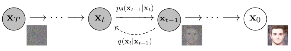
여기서 $x_0$은 원본 샘플, 즉 남자의 이미지입니다.
노이즈를 추가하는 과정은 오른쪽에서 왼쪽으로 가는 점선 화살표로 표시되며 그 과정은 $q(x_t|x_{t-1})$로 표시합니다. 최종적으로 $T$단계 후인 $x_T$에서는 노이즈만 납게됩니다.
생성 과정은 왼쪽에서 오른쪽으로, $x_T$에서 $x_0$으로 가는 실선 화살표로 표시되며 그 과정은 $p(x_{t-1}|x_t)$로 표시합니다. (머리 방향으로 구분하면 쉬울듯?)

Sampling

이 튜토리얼에서는 생성 과정을 쉽게 시각화할 수 있도록 매우 간단한 일차원 분포에서 샘플을 생성하는 방법을 배울 것입니다.
먼저 데이터를 생성하는 것부터 시작하겠습니다:

# @title 필요한 라이브러리 import
import matplotlib.pyplot as plt
import matplotlib as mpl
import pandas as pd
import numpy as np
import torch
import seaborn as sns
import itertools
from tqdm.auto import tqdm

# @title 데이터 분포 histogram
data_distribution = torch.distributions.mixture_same_family.MixtureSameFamily(
  torch.distributions.Categorical(torch.tensor([1, 2])),
  torch.distributions.Normal(torch.tensor([-4., 4.]), torch.tensor([1., 1.]))
)

dataset = data_distribution.sample(torch.Size([1000, 1]))
sns.histplot(dataset[:, 0])
plt.show()

output:

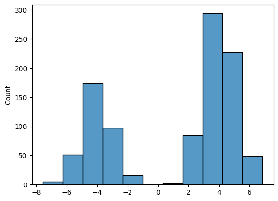
이 그래프는 데이터 분포, 즉 $q(x_0)$를 나타냅니다.
보시다시피, 훈련 데이터셋에는 두 개의 가우시안 분포가 혼합된 샘플이 포함되어 있으며, 오른쪽 구성 요소는 두 배 더 자주 샘플링 됩니다.

Forward Process과정은 논문의 방정식2에 나와 있습니다:

각 단계에 가우시안 노이즈를 추가:

이 분포의 평균과 편차는 최종 분포가 다음과 같도록 선택됩니다.
확산 과정 후에는 평균 0, 편차 1의 가우시안이 되며, 쉽게 샘플링 할 수 있습니다.

이 프로세스는 루프로 쉽게 구현됩니다:

# @title 파라미터 세팅
# we will keep these parameters fixed throughout
TIME_STEPS = 250
BETA = 0.02

# @title 확산 모델의 forward process
def do_diffusion(data, steps=TIME_STEPS, beta=BETA):
  # perform diffusion following equation 2
  # returns a list of q(x(t)) and x(t)
  # starting from t=0 (i.e., the dataset)

  distributions, samples = [None], [data]
  xt = data
  for t in range(steps):
    q = torch.distributions.Normal(
      np.sqrt(1 - beta) * xt,
      np.sqrt(beta)
    )
    xt = q.sample()

    distributions.append(q)
    samples.append(xt)

  return distributions, samples

# @title dataset 확산
_, samples = do_diffusion(dataset)

시간을 $x$축에 표시하고 확산된 샘플을 $y$축에 표시하여 확산 과정을 시각화할 수 있습니다:

# @title 확산 시각화
for t in torch.stack(samples)[:, :, 0].T[:100]:
  plt.plot(t, c='navy', alpha=0.1)
plt.xlabel('Diffusion time')
plt.ylabel('Data')
plt.show()

output:

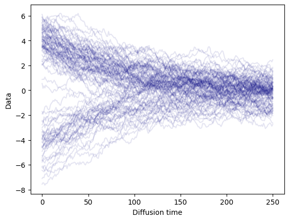
보시다시피 노이즈를 추가하면 모든 샘플이 점차 정규$\mathcal{N}(0,1)$분포로 변환되게 됩니다.
이제 이 과정을 반전시켜 모델을 학습시킬 수 있습니다.

Training

가능한 한 단순하게 하기 위해, 여기서는 논문에 나오는 식 3의 $L$를 그대로 사용합니다.
논문 후반에 소개된 여러 최적화 기법들은 실제 복잡한 현실 데이터셋에서만 중요한 역할을 하므로, 여기서는 적용하지 않았습니다.

이번 케이스에서 확산 모델은 먼저 훈련 예제를 손상시킨 다음 손상 과정의 각 단계에서 노이즈가 있는 예제를 통해 더 깨끗한 예제를 재구성하려고 시도하도록 훈련됩니다.
$L$는 음수 로그 확률의 상한선입니다:

Reverse Process(反転術式)를 수행하는 생성모델의 형태는 다음과 같습니다:

참고로 우리는 $\mu_{\theta}$와 $\Sigma_{\theta}$ 이 두개의 뉴럴 네트워크를 학습시키는데, 각각 노이즈가 더해진 샘플 $x_{t}$와 단계 $t$를 입력으로 받아 $x_{t-1}$의 얼마만큼의 노이즈가 추가되었는지(분포 되었는지) 예측합니다.
직관적으로, 우리는 각 확산 단계에서 $x_{t}$를 기반으로 계산되지 않은 $x_{t-1}$에 대한 예측을 최대화 할 수 있게 훈련시킵니다. 즉, $L$에서의 항 $p_{\theta}(x_{t-1}|x_{t})$는 각 확산 단계마다 등장한다는 뜻입니다.
꼭! $x_{t}$는 $x_{t-1}$에서 노이즈를 추가하여 생성되었다는 것, 그리고 네트워크는 그것을 되돌릴 방법을 학습한다는 것을 기억 해야 합니다. $L$에서 $q(x_{t}|x_{t-1})$과 관련된 다른 항들(foward_)은 좋은 생성 모델을 학습하기 위해 반드시 필요하지는 않습니다. (이 항들은상수이기 때문)
하지만 "perfect" 생성 모델이 $L$를 0으로 달성할 수 있도록 "frame of reference"로썬 유용합니다.

$L$는 아래와 같이 구현할 수 있습니다. 이 함수는 학습 샘플의 전체 확산 궤적과 역 과정을 정의할 두 개의 뉴럴 네트워크가 필요합니다:

# @title 손실 계산 합수, q와 p 필요
def compute_loss(forward_distributions, forward_samples, mean_model, var_model):
  # here we compute the loss in equation 3
  # forward = q , reverse = p

  # loss for x(T)
  p = torch.distributions.Normal(
    torch.zeros(forward_samples[0].shape),
    torch.ones(forward_samples[0].shape)
  )
  loss = -p.log_prob(forward_samples[-1]).mean()

  for t in range(1, len(forward_samples)):
    xt = forward_samples[t]         # x(t)
    xprev = forward_samples[t - 1]  # x(t-1)
    q = forward_distributions[t]    # q( x(t) | x(t-1) )

    # normalize t between 0 and 1 and add it as a new column
    # to the inputs of the mu and sigma networks
    xin = torch.cat(
      (xt, (t / len(forward_samples)) * torch.ones(xt.shape[0], 1)),
      dim=1
    )
    # compute p( x(t-1) | x(t) ) as equation 1
    mu = mean_model(xin)
    sigma = var_model(xin)
    p = torch.distributions.Normal(mu, sigma)

    # add a term to the loss
    loss -= torch.mean(p.log_prob(xprev))
    loss += torch.mean(q.log_prob(xt))

  return loss / len(forward_samples)

이제 평균과 분산을 예측하기 위해 두 가지 매우 간단한 신경망을 정의해 보겠습니다. 이 두 네트워크 모두 노이즈가 있는 샘플 $x_{t}$와 정규화된 시간 단계 $t$라는 두가지 입력을 받습니다. 위의 스니펫에서도 볼 수 있듯이 시간 단계는 추가적인 열로 추가되며, 입력도 1차원이므로 총 입력 크기는 2입니다.

# @title 평균_모델과 분산_모델 정의
# 평균_모델
mean_model = torch.nn.Sequential(
  torch.nn.Linear(2, 4), torch.nn.ReLU(),
  torch.nn.Linear(4, 1)
)
# 분산_모델
var_model = torch.nn.Sequential(
  torch.nn.Linear(2, 4), torch.nn.ReLU(),
  torch.nn.Linear(4, 1), torch.nn.Softplus()
)

이제 훈련을 해봅시다:

# @title 역전파/경사하강법 정의
# AdamW, weight decay(가중치 감쇠 루틴)가 분리되어 regularization에 더 유리함.
optim = torch.optim.AdamW(
  itertools.chain(mean_model.parameters(), var_model.parameters()),
  lr=1e-2, weight_decay=1e-6,
)
# 평균_모델과 분산_모델의 파라미터를 모두 하나로 합쳐 전달
# 두 네트워크 모두 학습

# @title 모델 훈련
loss_history = []
bar = tqdm(range(1000))
for e in bar:
  forward_distributions, forward_samples = do_diffusion(dataset)

  optim.zero_grad()
  loss = compute_loss(
    forward_distributions, forward_samples, mean_model, var_model
  )
  loss.backward()
  optim.step()

  bar.set_description(f'Loss: {loss.item():.4f}')
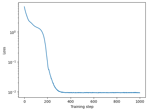
  loss_history.append(loss.item())

$L$를 검사하여 모델이 잘 수렴했는지 확인할 수 있습니다:

# @title loss값 확인
plt.plot(loss_history)
plt.yscale('log')
plt.ylabel('Loss')
plt.xlabel('Training step')
plt.show()

output:

Sample generation

최종적으로, 훈련된 신경망을 사용하여 데이터 분포에서 새로운 샘플을 생성할 수 있습니다.

이 과정은 이전의 확산 과정과 매우 유사하지만 차별점으로, 여기서는 정규 분포 $x_{T}$에서 시작하여 예측된 평균과 분산을 사용하여 점진적으로 노이즈를 "remove"합니다:

# @title 샘플 생성 정의 (reverse process)
def sample_reverse(mean_model, var_model, count, steps=TIME_STEPS):
  p = torch.distributions.Normal(torch.zeros(count, 1), torch.ones(count, 1))
  xt = p.sample()
  sample_history = [xt]
  for t in range(steps, 0, -1):
    xin = torch.cat((xt, t * torch.ones(xt.shape) / steps), dim=1)
    p = torch.distributions.Normal(
      mean_model(xin), var_model(xin)
    )
    xt = p.sample()
    sample_history.append(xt)
  return sample_history

# @title 샘플 생성
samps = torch.stack(sample_reverse(mean_model, var_model, 1000))

# @title 시각화
for t in samps[:,:,0].T[:200]:
  plt.plot(t, c='C%d' % int(t[-1] > 0), alpha=0.1)
plt.xlabel('Generation time')
plt.ylabel('Data')
plt.show()

output:

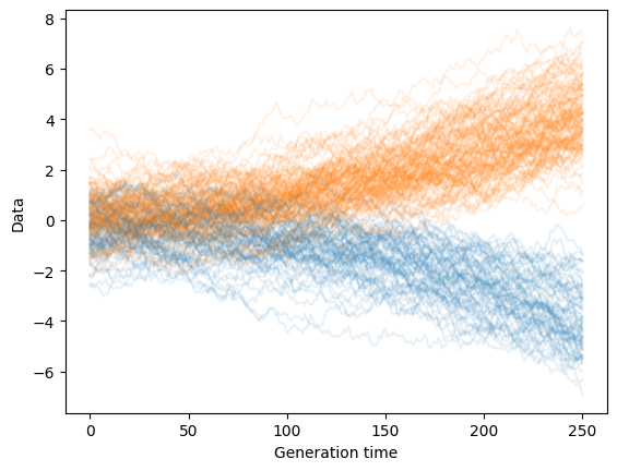
그리고 이것이 생성 마지막 단계에서의 분포입니다:

# @title generated_histogram
sns.histplot(samps[-1, :, 0])
plt.show()

output:

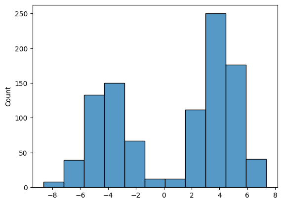
초기 데이터 분포와 매우 유사하므로, 우리 모델이 훈련 데이터셋과 유사한 샘플을 생성하는 방법을 성공적으로 학습했음을 의미합니다!