Chapter 2. Simple Linear Regression

Regression Analysis

Study a functional relationship between variables

• response variable y(dependent variable)
• explanatory variable x(independent variable)

Simple linear regression model

• When $E(Y)$ is a linear function of parameters, the models is called a linear statistical model.
• Simple linear regression model : $E(Y)=\beta_0+\beta_1x$
  

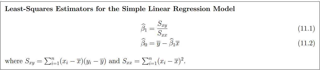
Method of estimation

Sum of squares for error(SSE)

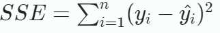
• The least squares estimators $\hat{\beta_0}$ and $\hat{\beta_1}$ are the estimators of $\beta_0$ and $\beta_1$ that minimize the sum of squares for error $SSE(\beta_0,\beta_1)$
  

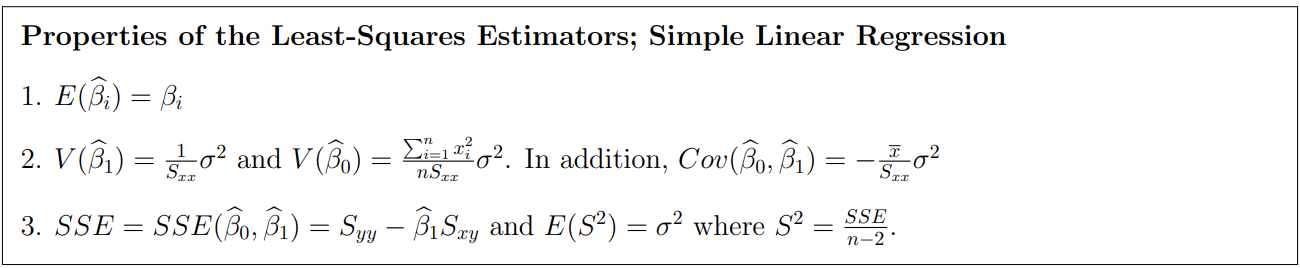
Method of inference

• Consider a simple linear regression model : $Y=\beta_0+\beta_1x+\epsilon$

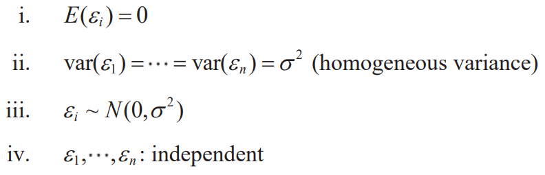
• Assumption

  • $E(\epsilon) = 0$
  • $V(\epsilon) = \sigma^2$ that does not depend on $x$
  • Suppose $n$ independent observations are to be made on this model
    : $Y_i = \beta_0+\beta_1x_i+\epsilon_i$

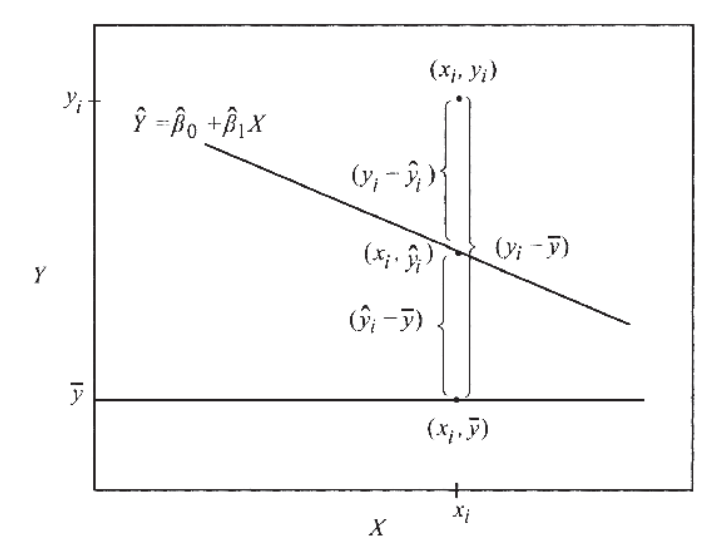
Measuring the quality of fit

Decomposition of Sum of Squares

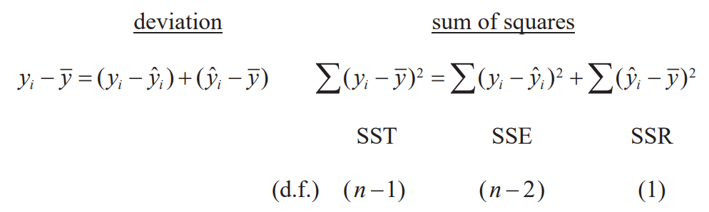
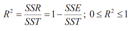
Coefficient of determination

• $R^2$ : Proportion of variation of y explained by x
  

Chapter 3. Multiple Linear Regression

• Multiple linear regression model : $E(Y)=\beta_0+\beta_1x_1 + ... + \beta_kx_k$

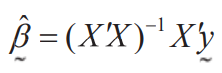
Least squares estimates

• minimize $\sum_{i=1}^{n}(y_i - \beta_0 - \beta_1x_{i1} - ... - \beta_px_{ip})^2$
• normal equation : $e_i = y_i - (\hat{\beta_0}+\hat{\beta_1}x_{i1}+...+\hat{\beta_p}x_{ip}) = y_i- \hat{y_i}$
• estimate of $\sigma^2$ : $\frac{1}{n-p-1}\sum_{i=1}^{n}(y_i- \hat{y_i})^2 = \frac{1}{n-p-1}SSE$

Matrix approach

Method of inference

Properties of estimates

Recall that

Measuring the quality of fit

Decomposition of sum of squares

Multiple correlation coefficient(MCC) & Adjusted MCC

• $R^2 \uparrow 1$ means that determination of y by linear combination of x becomes larger or proportion of variation of y explained by x1,...,xp
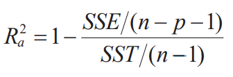
• As the number of explanatory variables increases, $R^2$ always increases and $SSE$ unconditionally decreases.
• $R^2$ is inappropriate for comparing the fitness between models with different numbers of explanatory variables. Therefore, consider the following adjusted $R^2$
  

Interpretations of regression coefficients

$y_i = \beta_0 + \beta_1x_{i1} + ... + \beta_px_{ip} + \epsilon_i$

• $\beta_0$(constant coef.) : the value of y when $x_1=x_2=...=x_p=0$
• $\beta_j$(regression coef.) : the change of y corresponding to a unit change in $x_j$ when $x_i$'s are hold constant(fixed)

Chapter 4. Regression Diagnostics: Detection of Model Violations

Validity of model assumption

$y_i = \beta_0 + \beta_1x_{i1} + ... + \beta_px_{ip} + \epsilon_i$, $\epsilon_i \sim iid N(0,\sigma^2)$

Linearity assumption

$\Rightarrow$ graphical methods(scatter plot for simple linear regression)

Error distribution assumption

$\Rightarrow$ graphical methods based on residuals

Assumptions about explanatory variables

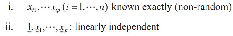
$\Rightarrow$ graphical methods or correlation matrices

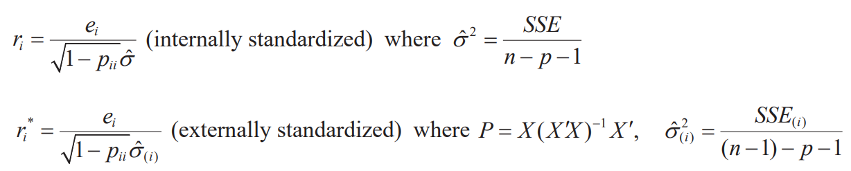
Residuals

• If a regression equation is obtained from the population, the difference between the predicted value and the actual observed value obtained through the regression equation is error
• On the other hand, if a regression equation was obtained from the sample group, the difference between the predicted value and the actual observed value obtained through the regression equation is the residual
  

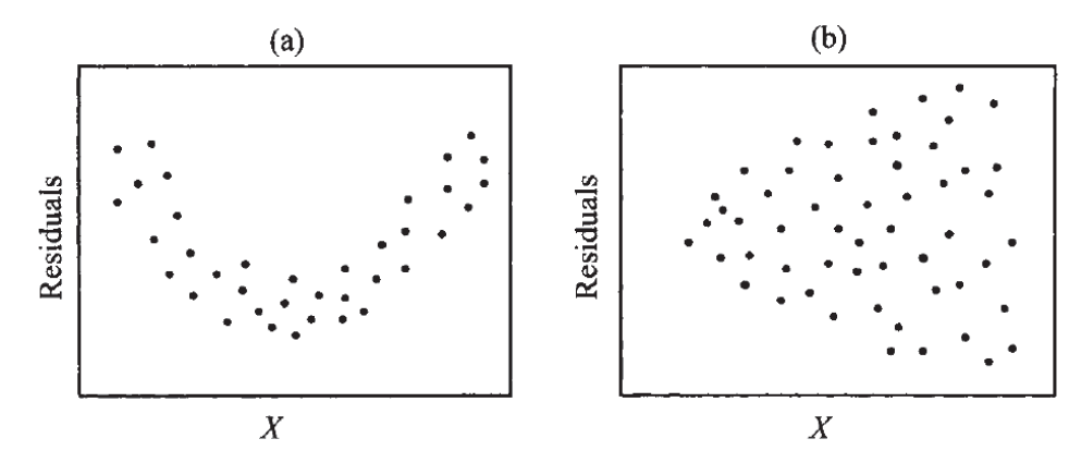
Residual plot

$(x_1,r)/.../(x_p,r)$ plot

• If the assumptions hold, this should be a random scatter plot
• Tools for checking non-linearity / non-homogeneous variance
  

Scatter plot

• $(x_{i1}, y_i), ..., (x_{ip}, y_i)$ for linearity assumption
• $(x_{il},x_{im})(l\neq m)$ for linear independence(multicollinearity)

Leverage, Influence and Outliers

• Leverage : Checking outliers in explanatory variables
• Measures of influence : Cook's distance, Difference in Fits, Hadi's measure & Potential-Residual Plot
• Outliers : Leverage(outliers in the predictors), Standardized(studentized) residual(outliers in the response variable)

Chapter 5. Qualitative Variable as Predictors

• Sometimes, it is necessary to use qualitative(or categorical) variable in a regression through indicator(dummy) variables

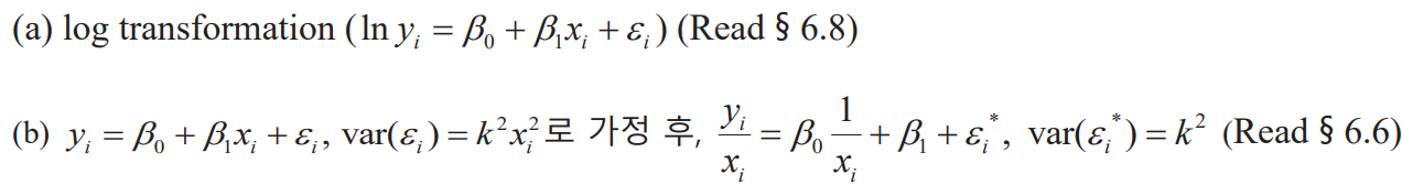
Chapter 6. Transformation of Variables

• Use transformation to achieve linearity and/or homoscedasticity
  
  

Variance stabilization transformation

• The distribution of $Y|x$ may not be a normal distribution.
• Therefore, $E(Y|x)$ and $V(Y|x)$ may have a functional relationship with each other. Example: Poisson distribution, binomial distribution, negative binomial distribution
• When the distribution of $Y|x$ or the functional relationship between $E(Y|x)$ and $V(Y|x)$ can be known, a special transformation can satisfy the assumption of the normal distribution and eliminate the functional relationship.
• Log transformation is typically used a lot to reduce variance

Chapter 7. Weighted Least Squares(WLS)

$\Rightarrow$ Residual plot shows the empirical evidence of heteroscedasticity(이분산성)

Strategies for treating heteroskedasticity

• Transformation of variable
  
• WLS
  
• (b) of Transformation of variables gives the same result as WLS, but it is difficult to interpret the result.

Weighted Least Squares(WLS)

• We use WLS when we suspect an equally distributed assumption of error.
• It is used when you want to create a regression model that is less affected by outliers.
  
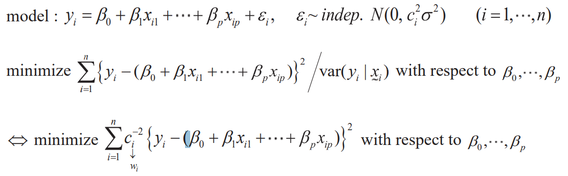
• Idea
  - Incorrect observations adjust the weight to have less effect on the min of SSE
  - If $w_i=0$, the observation is excluded from the estimation and is the same as OLS if all $w_i$ are equal.

Sums of Squares Decomposition in WLS

Chapter 8. The Problem of Correlated Errors

• Assumption of independence in the regression model: the error terms $e_i$ and $e_j$ are not correlated with each other. $Cov(e_i,e_j)=0, i \neq j$
• Autocorrelation
  - The correlation when the observations have a natural sequential order
  • Adjacent residuals tend to be similar in both temporal and spatial diemensions(economic time series)

Effect of Autocorrelation of Errors on Regression Analysis

• The efficiency of LSE for regression coefficients is poor(unbiased but no minimum variance)
• $\sigma^2$ or the s.e. of the regression coefficient may be underestimated. In other words, the significance of the regression coefficient is overestimated
• Commonly used confidence intervals or significance tests are no longer valid

Two types of the autocorrelation problem

• Type 1: autocorrelation in appearance(omission of a variable that should be in the model)
  $\rightarrow$ Once this variable is uncovered, the problem is resolved
• Type 2: pure autocorrelation
  $\rightarrow$ involving a transformation of the data

How to detect the correlated errors?

• residuals plot(index plot) : a particular pattern
• runs test, Durbin-Watson test

What to do with correlated errors?

• Type 1: consider another variables if possible
• Type 2: consider AR model to the error $\rightarrow$ reduce to a model with uncorrelated error

Numerical evidences of correlated errors

Runs test

• uses signs(+,-) of residuals
• Run: repeated occurrence of the same sign
• NR: # of runs
• Idea: NR $\uparrow$ if negative corr, NR $\downarrow$ if positive corr

Durbin-Watson test(a popular test of autocorrelation in regression analysis)

• Use it under the assumption called as AutoRegressive model of order 1(AR1)
  
• Durbin-Watson's statistic & Estimator of autocorrelation
  
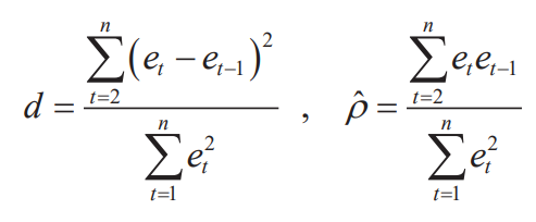
• Idea: small values of $d$ is positive correlation & large values of $d$ is negative correlation

Chapter 9. Analysis of Collinear Data

• Interpretation of the multiple regression equation depends implicitly on the assumption that the predictor variables are not strongly interrelated
• If the predictors are so strongly interrelated, the regression results are ambiguous : problem of collinear data or multicollinearity

Multicollinearity(다중공선성)

• Regression assumption: rank(X)=p+1
• Multicollinearity is not found through residual analysis.
• The cause of multicollinearity may be a lack of observation or the uniqueness of the independent variables to be analyzed
• The multicollinearity problem is considered after regression diagnosis including residual analysis

Symptom of multicollinearity

1. Model is significant byt some of $x_i$ are not significant
2. Estimation of $\hat{\beta_i}$ are unstable and drastic change of $\hat{\beta_i}$ by adding or deleting a variable
3. Estimation result contrary to the common sense

Numerical measure of multicollinearity

Correlation coefficients of $x_i$ and $x_j (i \neq j)$

• Pairwise linear relation but can't detect linear relation among 3 or more variables

Variance Inflation Factor(VIF)

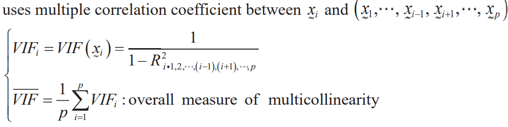
• VIF>10 evidence of multicollinearity

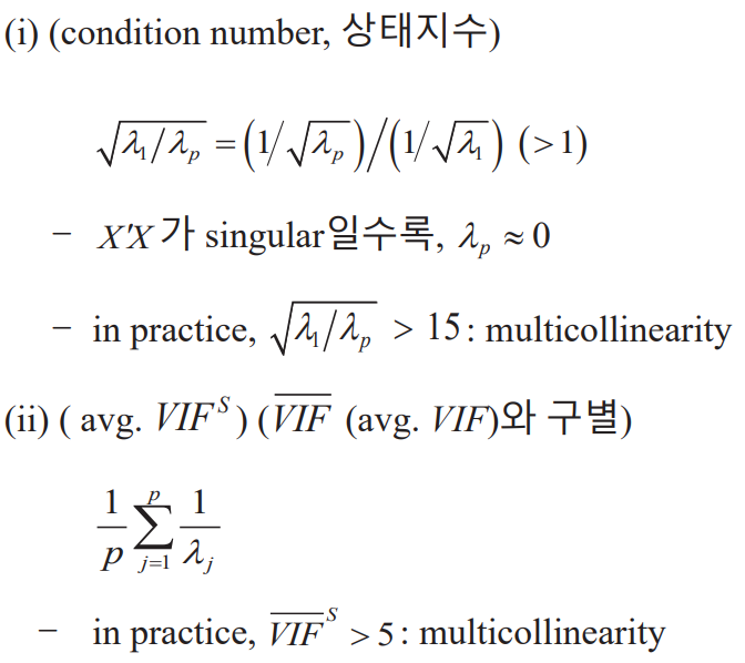
Principal components

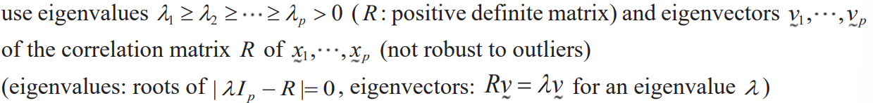
• Overall measure of multicollinearity
  

What to do with multicollinearity data

• (Experimental situation) : design an experiment so that multicollinearity does not occur
• (Observational situation) : reduce the model(essentially reduce the variables) using the information from the PC's, Ridge regression

Chapter 11. Variable Selection

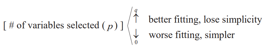
• Goal: to explain the response with the smallest number of explanatory variables
• Balancing between goodness of fit and simplicity
  

Statictics used in Variable Selection

• To decide that one subset is better than another, we need some criteria for subset selection
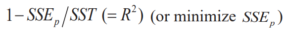
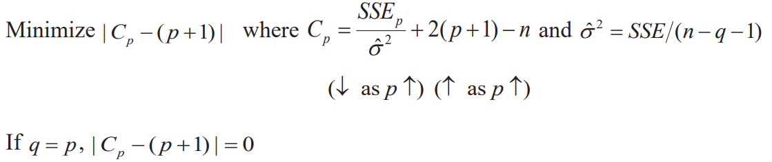
• The criteria is minimizing a modified $SSE_p$

Adjusted multiple correlation coefficient

• For fixed p, maximize among possible choices of p variables
  
• For different p's, maximize
  

Mallow's $C_p$

AIC

BIC

Partial F-test statistics for testing

Variable Selection

1. Evaluating all possible equations
   
2. Variable selection precedures(Partial F-test)
   

• Forward selection
• Backward elimination
• Stepwise selection

Chapter 12.Logistic Regression

• Dependent variable:Quanlitative & Independent variables:Quantitative or Qualitative

Modeling Qualitative Data

• Rather than predicting these two values of the binary response variable, try to model the probabilities that the response takes one of these two values
• Let $\pi$ denote the probability that Y=1 when X=x
• Logistic model
  
  
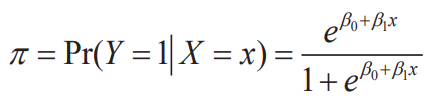
• Logistic regression function(logistic model for multiple regression)
  
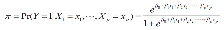
• Nonlinear in the paramters but it can be linearized by the logit transformation
  
• Odds : Indicates how many times the probability of success is that of failure
  
• Logit
  
• Modeling and estimating the logistic regression model
  - Maximum likelihood estimation
  • No closed-form expression exists for the estimates of the parameters. To fit a logistic regression in practice a computer program is essential
  • Information criteria as AIC and BIC can be used for model selection
  • Instead of SSE, the logarithm of the likelihood for the fitted model is used

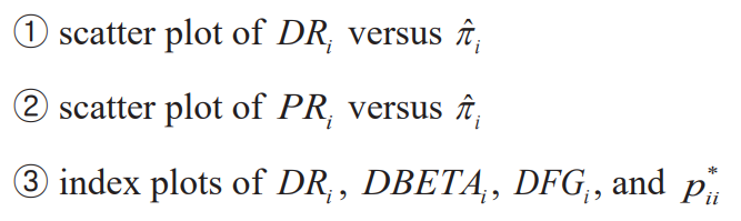
Diagnostics in logistic regression

• Diagnostic measures
  
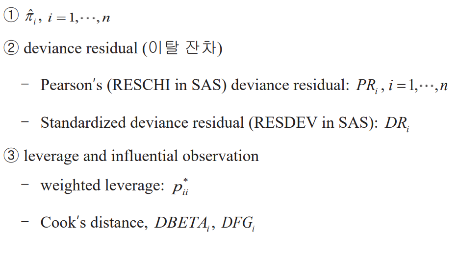
• How to use the measures: same way as the corresponding ones from a linear regression