
Chapter 2. 분류 알고리즘의 기초
2장 목표
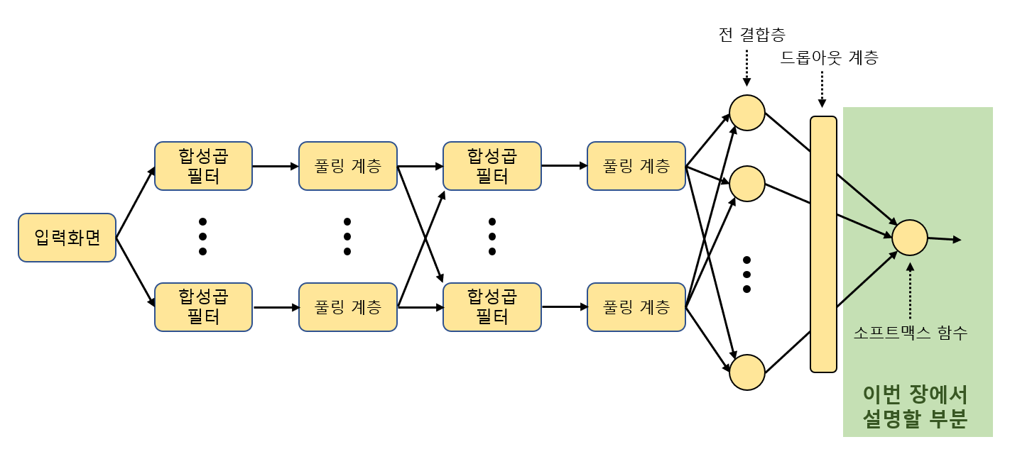
- CNN의 전체 모습 중 가장 오른쪽의 '소프트맥스 함수'의 역할 알기
- '선형 분류기(linear classifier', '퍼셉트론(perceptron)'이라고 하는 노드의 역할 알기
2.1 로지스틱 회귀를 이용한 이항 분류기
2.1.1 확률을 이용한 오차 평가
바이러스에 감염되었을 확률을 예로 하면
특정 바이러스의 감염을 조사하는 예비 검사 결과가 두 종류의 수치로 되어있고 각각의 결과에 대해 실제로 감염되어있는지 나타낸다.
이를 기반으로 새로운 결과 가 나왔을 때 이 환자가 실제로 감염되었는지를 판정하는 것이 목표
환자가 바이러스에 감염되었을 확률
평면을 분할하는 직선
는 시그모이드 함수 (0~1까지 완만하게 변화하는 함수)
주어진 데이터가 총 개일 때,
번째 데이터를 ,
번째 데이터를 바르게 예측할 확률을 이라고 하면
개의 데이터가 모드 정답일 확률
가 변하면 위의 식도 변하기 때문에
이 확률이 파라미터를 평가하는 기준이 된다.
최우추정법에 의해 확률이 높은 쪽의 데이터에 최적화된 것
최우추정법(Maximum likehood method)
- 주어진 데이터를 바르게 예측할 확률을 최대화 하는 것
하지만 곱셈을 대량으로 하는 것은 텐서플로에서 계산 효율이 좋지 않다.
따라서 오차 함수 를 최소화 하도록 파라미터를 정한다. (로그함수의 성질 이용)
2.1.2 텐서플로를 이용한 최우추정 실행
앞의 내용을 텐서플로 코드로 실행
import tensorflow.compat.v1 as tf
tf.disable_v2_behavior()
import numpy as np
import matplotlib.pyplot as plt
from numpy.random import multivariate_normal, permutation
import pandas as pd
from pandas import DataFrame, Series

np.random.seed(20160512) #난수 패턴 지정

#t=0인 데이터를 난수로 생성 (비감염)
n0, mu0, variance0 = 20, [10, 11], 20
data0 = multivariate_normal(mu0, np.eye(2)*variance0 ,n0)
df0 = DataFrame(data0, columns=['x1','x2'])
df0['t'] = 0

#t=1일 데이터를 난수로 생성 (감염)
n1, mu1, variance1 = 15, [18, 20], 22
data1 = multivariate_normal(mu1, np.eye(2)*variance1 ,n1)
df1 = DataFrame(data1, columns=['x1','x2'])
df1['t'] = 1

#모든 데이터를 하나로 모아 행의 순번을 무작위로 변경
df = pd.concat([df0, df1], ignore_index=True)
train_set = df.reindex(permutation(df.index)).reset_index(drop=True)
train_set.head()

#데이터 형태를 다차원 배열(행렬)로 변환
train_x = train_set[['x1','x2']].values
train_t = train_set['t'].values.reshape([len(train_set), 1])

x = tf.placeholder(tf.float32, [None, 2])
w = tf.Variable(tf.zeros([2, 1]))
w0 = tf.Variable(tf.zeros([1]))
f = tf.matmul(x, w) + w0  #브로드캐스팅 규칙 사용
p = tf.sigmoid(f)

t = tf.placeholder(tf.float32, [None, 1])
loss = -tf.reduce_sum(t*tf.log(p) + (1-t)*tf.log(1-p)) #오차함수 E = loss
train_step = tf.train.AdamOptimizer().minimize(loss)   #loss최소화

#정답률
correct_prediction = tf.equal(tf.sign(p-0.5), tf.sign(t-0.5))
accuracy = tf.reduce_mean(tf.cast(correct_prediction, tf.float32))

sess = tf.Session()
sess.run(tf.initialize_all_variables())

#경사 하강법에 의한 파라미터 최적화 2만회 반복
i = 0
for _ in range(20000):
    i += 1
    sess.run(train_step, feed_dict={x:train_x, t:train_t})
    if i % 2000 == 0:
        loss_val, acc_val = sess.run(
            [loss, accuracy], feed_dict={x:train_x, t:train_t})
        print ('Step: %d, Loss: %f, Accuracy: %f'
               % (i, loss_val, acc_val))

#이 시점 파라미터 출력
w0_val, w_val = sess.run([w0, w])
w0_val, w1_val, w2_val = w0_val[0], w_val[0][0], w_val[1][0]
print(w0_val, w1_val, w2_val)

#추출값 이용해 결과를 그래프로 표시
train_set0 = train_set[train_set['t']==0]
train_set1 = train_set[train_set['t']==1]

fig = plt.figure(figsize=(6,6)) #그래프의 사이즈
subplot = fig.add_subplot(1,1,1) #그래프가 그려지는 위치 나타냄 (여러 개의 그래프 그릴때 사용가능)
subplot.set_ylim([0,30])
subplot.set_xlim([0,30])
subplot.scatter(train_set1.x1, train_set1.x2, marker='x')
subplot.scatter(train_set0.x1, train_set0.x2, marker='o')

linex = np.linspace(0,30,10) #배열만들기 (start, stop, 총 갯수) == 정의역
liney = - (w1_val*linex/w2_val + w0_val/w2_val)
subplot.plot(linex, liney) #직선f(x_1, x_2)=0 그림

field = [[(1 / (1 + np.exp(-(w0_val + w1_val*x1 + w2_val*x2))))
          for x1 in np.linspace(0,30,100)]
         for x2 in np.linspace(0,30,100)]

subplot.imshow(field, origin='lower',
               cmap=plt.cm.gray_r, alpha=0.5)
위의 코드에서 쓰인 시그모이드 함수
이를 로지스틱 함수(logistic function)라 하며,
이 분석 방법은 로지스틱 회귀(logistic regression)라고 함
2.1.3 테스트 세트를 이용한 검증
오버피팅(overfitting)
- 머신러닝에서 중요한 것은 미지의 데이터에 대한 예측 정확도를 향상시키는 것인데 트레이닝 세트 데이터만 갖는 특징에 대해 과잉 최적화가 발생할 수 있음
- 트레이닝 세트에 대한 정답률을 높지만 미지의 데이터의 예측 정확도는 낮은 경우가 오버피팅
- 오버피팅을 피하기 위해선 트레이닝 세트의 데이터 중 일부 데이터를 테스트용으로 나누어 놓는 방법이 있음
- ex) 80%의 데이터로 트레이닝하면서 20%의 데이터에 대한 정답률 변화 살펴봄
앞의 코드 일부를 수정해 트레이닝 세트와 테스트 세트 각각에 대한 정답률 변화 확인
#난수 생성 후 80%는 데이터 세트로, 20%는 테스트 세트로 나눔
#(기본 데이터 양의 40배)
np.random.seed(20160531)


n0, mu0, variance0 = 800, [10, 11], 20
data0 = multivariate_normal(mu0, np.eye(2)*variance0 ,n0)
df0 = DataFrame(data0, columns=['x','y'])
df0['t'] = 0

n1, mu1, variance1 = 600, [18, 20], 22
data1 = multivariate_normal(mu1, np.eye(2)*variance1 ,n1)
df1 = DataFrame(data1, columns=['x','y'])
df1['t'] = 1

df = pd.concat([df0, df1], ignore_index=True)
df = df.reindex(permutation(df.index)).reset_index(drop=True)

num_data = int(len(df)*0.8)
train_set = df[:num_data]
test_set = df[num_data:]

train_x = train_set[['x','y']].values
train_t = train_set['t'].values.reshape([len(train_set), 1])
test_x = test_set[['x','y']].values
test_t = test_set['t'].values.reshape([len(test_set), 1])

#전과 동일
x = tf.placeholder(tf.float32, [None, 2])
w = tf.Variable(tf.zeros([2, 1]))
w0 = tf.Variable(tf.zeros([1]))
f = tf.matmul(x, w) + w0
p = tf.sigmoid(f)

t = tf.placeholder(tf.float32, [None, 1])
loss = -tf.reduce_sum(t*tf.log(p) + (1-t)*tf.log(1-p))
train_step = tf.train.AdamOptimizer().minimize(loss)

correct_prediction = tf.equal(tf.sign(p-0.5), tf.sign(t-0.5))
accuracy = tf.reduce_mean(tf.cast(correct_prediction, tf.float32))

sess = tf.Session()
sess.run(tf.initialize_all_variables())

train_accuracy = []
test_accuracy = []
for _ in range(2500):
    sess.run(train_step, feed_dict={x:train_x, t:train_t})
    acc_val = sess.run(accuracy, feed_dict={x:train_x, t:train_t})
    train_accuracy.append(acc_val)
    acc_val = sess.run(accuracy, feed_dict={x:test_x, t:test_t})
    test_accuracy.append(acc_val)

#그래프 그리기
fig = plt.figure(figsize=(8,6))
subplot = fig.add_subplot(1,1,1)
subplot.plot(range(len(train_accuracy)), train_accuracy,
             linewidth=2, label='Training set')
subplot.plot(range(len(test_accuracy)), test_accuracy,
             linewidth=2, label='Test set')
subplot.legend(loc='upper left')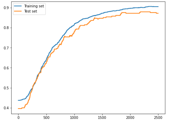
오버피팅이 발생한 경우에는 테스트 세트에 대한 정답률이 트레이닝 세트에 대한 정답률보다 더 높게 증가하지 않음
- 트레이닝 세트 데이터에 대해서만 최적화가 이루어지기 때문

🐥공부 기록 블로그🐥