Designing algorithms

The divide-and-conquer approach

1. Divide-and-Conquer

• Many recursive algorithms follow a divide-and-conquer approach
• Three steps at each level of the recursion
  • Divide

    Divide the problem into a number of subproblems that are smaller instances of the same problem

  • Conquer

    Conquer the subproblems by solving them recursively. If the subproblem sizes are small enough, however, just solve the subproblems in a straightforward manner.

  • Combine

    Combine the solutions to the subproblems into the solution for the original problem

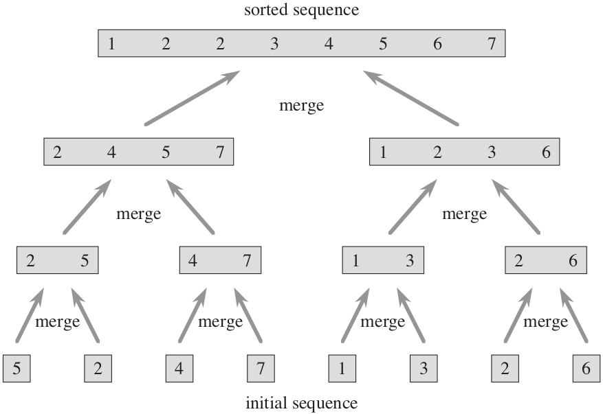
• The merge sort algorithm colsely follows the divide-and-conquer paradigm
  • Divide

    Divide the $n$-element sequence to be sorted into two subsequences of $n$/2 elements each

  • Conquer

    Sort the two subsequences recursively using merge sort

  • Combine

    Merge the two sorted subsequences to produce the sorted answer

2. Merge procedure

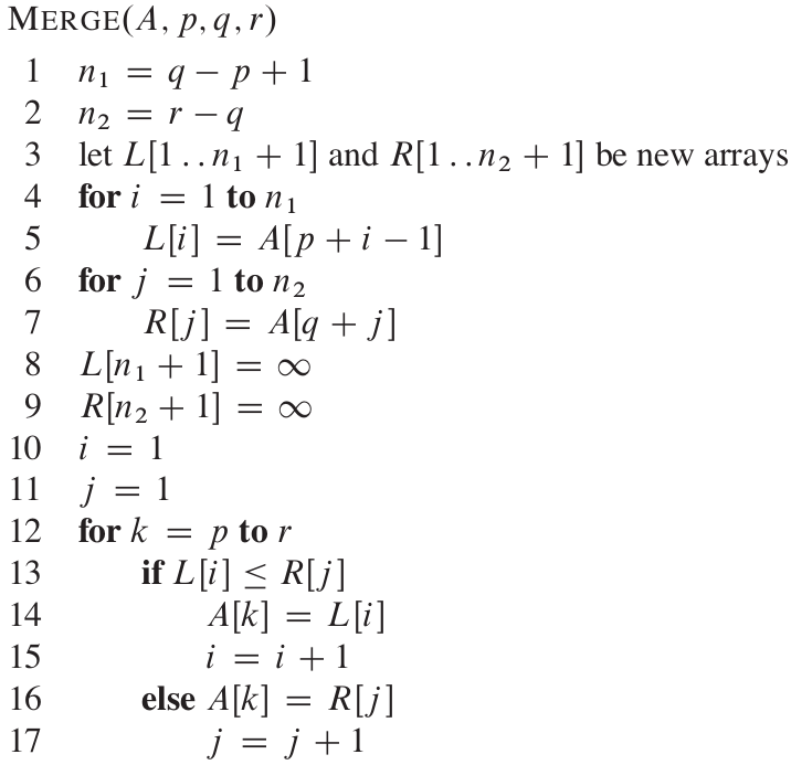
• $A$ is an array and $p, q,$ and $r$ are indices into the array such that $p \leq q < r$

• The subarrays $A[p \dots q]$ and $A[q+1 \dots r]$ are in sorted order

• It merges the two subarrays to form a single sorted subarray that replaces the current subarray $A[p \dots r]$

• This procedure takes time $\Theta(n)$, where $n = r - p + 1$ is the total number of elements being merged

• $\infty$ is sentinel value, so that whenever a value with $\infty$ is exposed, it cannot be the smaller value unless both subarrays have their sentinel value exposed

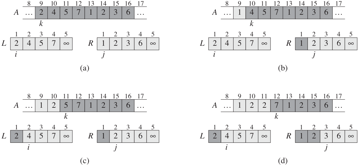
• The operation of lines 10-7 in the call MERGE$(A, 9, 12, 16)$

  
  

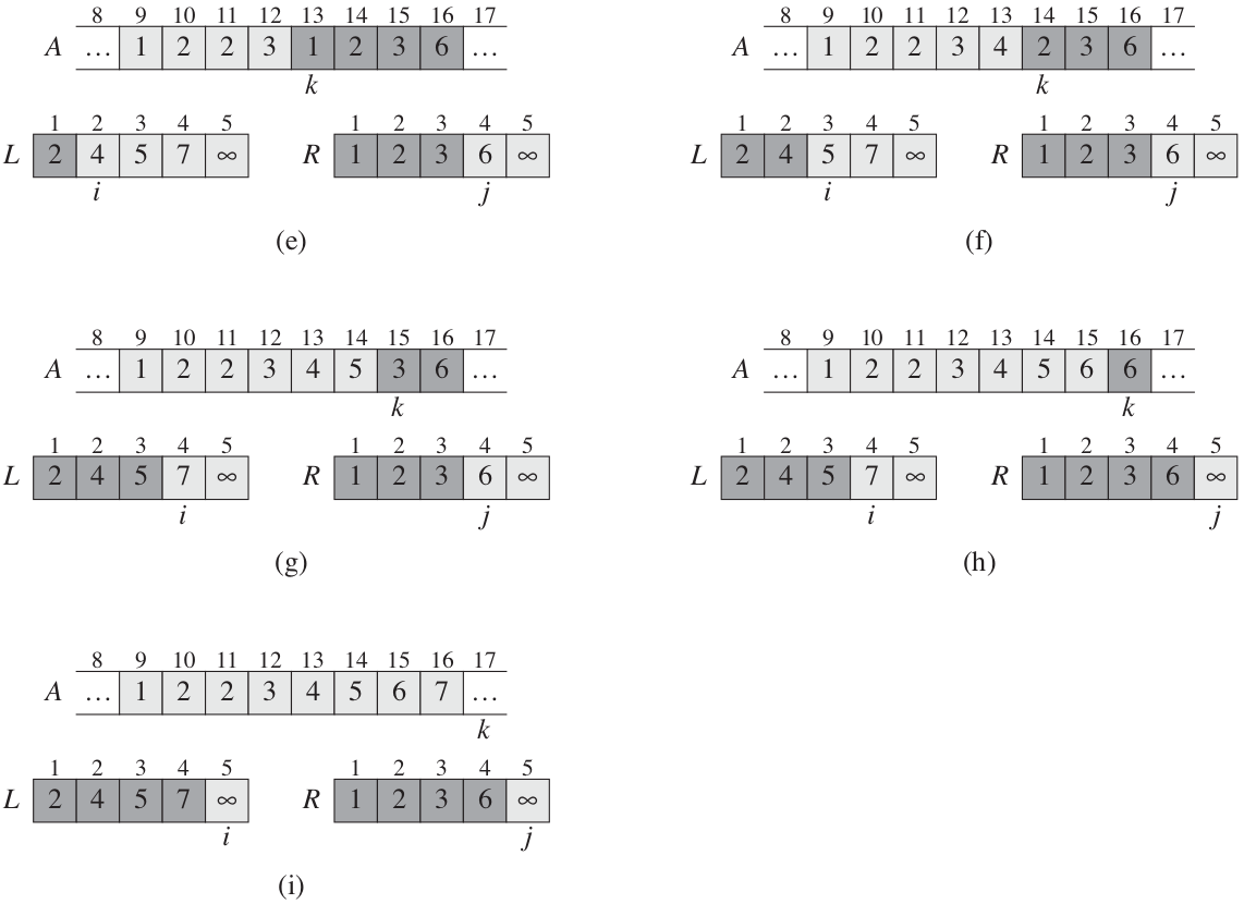
• Loop invariant

  At the start of each iteration of the for loop of lines 12-17, the subarray $A[p \dots k - 1]$ contatins the $k - p$ smallest elements of $L[1 \dots n_1 + 1]$ and $R[1 \dots n_2 + 1]$, in sorted order. Moreover, $L[i]$ and $R[j]$ are the smallest elements of their arrays that have not been copied back into $A$.

  • Initialization

    Prior to the first iteration of the loop, we have $k = p$, so that the subarray $A[p \dots k - 1]$ is empty. This empty subarray contains the $k - p = 0$ smallest elements of $L$ and $R$, and since $i = j =1$, both $L[i]$ and $R[j]$ are the smallest elements of their arrays that have not been copied back into A.

  • Maintenance

    Let it first suppose that $L[i] \leq R[j]$. Then $L[i]$ is the smallest element not yet copied back into $A$. Because $A[p \dots k - 1]$ contains the $k - p$ smallest elements, after line 14 copies $L[i]$ into $A[k]$, the subarray $A[p \dots k]$ will contain the $k - p + 1$ smallest elements. Incrementing $k$ and $i$ reestablishes the loop invariant for the next iteration. If instead $L[i] > R[j]$, then lines 16-17 perform the appropriate action to maintain the loop invariant.

  • Termination

    At termination, $k = r + 1$. By the loop invariant, the subarray $A[p \dots k - 1]$, which is $A[p \dots r]$, contains the $k - p = r - p + 1$ smallest elements of $L[1 \dots n_1 + 1]$ and $R[1 \dots n_2 + 1]$, in sorted order. The arrays $L$ and $R$ together contain $n_1 + n_2 + 2 = r - p + 3$ elements. All but the two largest have been copied back into A, and these two largest elements are the sentinels.

3. Merge sort algorithm

• The MERGE-SORT$(A, p, r)$ sorts the elements in the subarray $A[p \dots r]$
• If $p \geq r$, the subarray has at most one element and is therefore already sorted
• An index $q$ partitions $A[p \dots r]$ into two subarrays: $A[p \dots q]$, containing $\lceil n/2 \rceil$ elements, and $A[q + 1 \dots r]$, containing $\lfloor n/2 \rfloor$ elements
• The operation of merge sort on the array $A = \langle 5,2,4,7,1,3,2,6 \rangle$