Abstract
By using Diffusion Probabilistic models, high quality image synthesis is made possible. The best performing method is training on weighted variantional bound. The variantional bound comes from connecting 1. [Diffusion Probabilistic model] and 2. [denoising score matching through Langevin dynamics]. The proposed model is a lossy decompression in a progressive manner and it can be interpreted as a generalization of autoregressive decoding. The implementation is available at github.
Prerequisite
What is Diffusion?
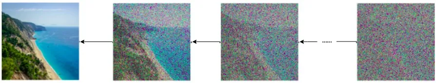
Diffusion came from the term used in Thermodynamics, where particle or molecules spontaneously move from high concentration to low concentration. Likening an image to a liquid, its pixels act like an atom. We repricate the physical diffusion process with noise. Adding noise to the image is like the diffusion process. By gradually adding noise at successive individual steps we are destorying the information. And we call this Forward Diffusion Process. The second part of the task is to restore the image by gradually denoising it. This denoising is called the Backward Diffusion Process.
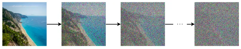
Forward Process is fundamentally a process where a transform function transforms a complex distribution to a predefined prior distribution.
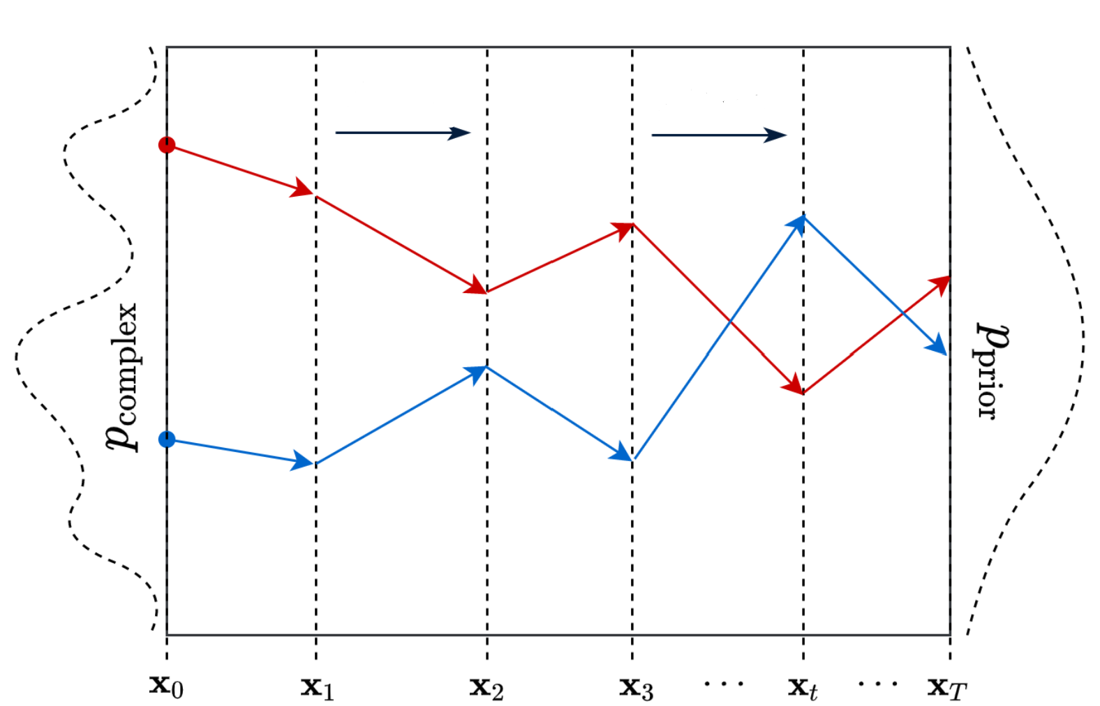 The data points on a complex distribution are mapped to a point on a prior distribution. The data points on a complex distribution are mapped to a point on a prior distribution. | 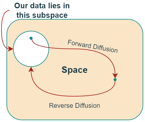 A high-level conceptual overview of the entire image space. A high-level conceptual overview of the entire image space. |
|---|
In DDPM the prior distribution is defined to follow a Gaussian distribution and the transformation mechanism is assumed to be a Markov Chain Process, meaning that the current state only depends on the one step previous state and the transition probability between states. Lets start with notations first.
- X : Random variable for an image distributed according to probability distribution complex P(x)
- so X=x for some image from the possible set of Images in X.
- n : Number of pixels in a image(HxW of pixels).
- Then X is a set of N random variables i.e, X={} and for N pixel image.
Markov Chains and what it means to have them in DDPMs
Given that a image state at timestep K is represented as Xk, the forward path can be written as follows. Thus by the property of Markov process, the output of the current time step is conditioned is only on t-1 timestep.
In the context of diffusion process, the number of timesteps T is the number of steps needed to convert input image into a pure gaussian noise. If the Backward process is exactly the opposite of the forward process, Then it would be represented as follows.
Deep dive into DDPM
Forward Step
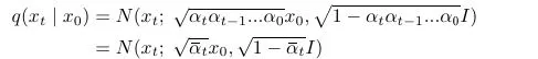
Diffusion model can be understood as a lantent variable model which get an input image and maps it to the latent space using fixed forward diffusion process q. q process is a Markov chain and the goal of the forward q process is to add noise progressively to get an approximate posterior q(x1:T|x0) where each xi is regarded as latent variables having the same dimensionality as input x0.
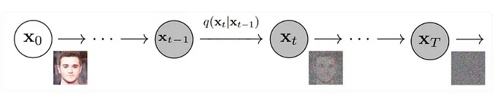
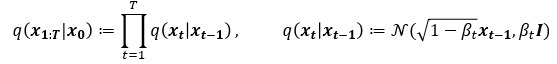
The total noise adding process is a joint distribution of Markov chain gradually adding Gaussian noise. The interesting part of forward process is that the variance is a hyperparameter not a trainable parameter. The reason why the mean and the variance of the Gaussian distribution has the particular form is due to when is small enough (Meaning that is very small).
Backward Step
The backward diffusion process, the model tries to learn the reverse denoising process of recovering the original form of the input.
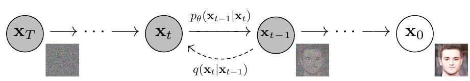
As mentioned earlier, is a very small value. This also implies that reverse process can be estimated as a Gaussian distribution and ,the estimation of the real distribution q, can be chosen to be Gaussian as well as parameterize the mean and variance as
starting from a pure Gaussian noise: . The whole denoising process of is given as by the Markov Assumption. Finally this chain of equations can be simplified to a product form().
Evidence lower Bound
The objective of the generative model is to model the probability distribution of the data or . The original data space is intractable leading us to instead learn approximate distribution
Now to maximize the likelihood of , we optimize the negative log likelihood of it. By Jensen's inequality the NLL of p is described as below.
Minimizing the righthand side of the equation will minimize the evidence upper bound. Thus the objective of the the training:
We do not know the conditional distribution using the Transfer from to during process for generation. By Bayes rule,
This q(xt) is intractable because the distribution of 1) each time-step and 2) depends on the entire data distribution space of all possible images. Instead we make a Neural Network learn a distribution given approximating to . With KL divergence, calculating the distance between P and Q is done.
KL divergence can be written as
which can also be formulated as an expectation
Computing the loss
After some simplification the final term can be as below.
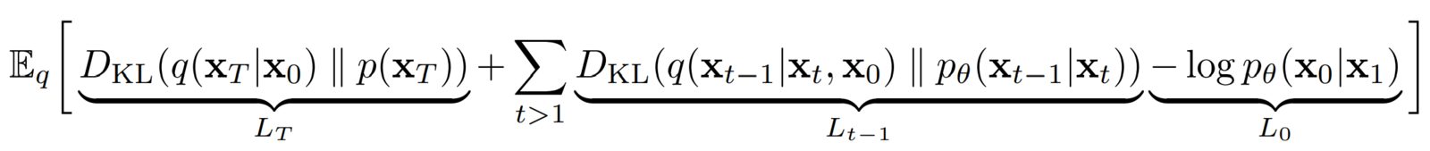
The terms below were ignored
– The authors got better results without this.
– This is the “KL divergence” between the distribution of the final latent in the forward process and the first latent in the reverse process. However, there are no neural network parameters involved here, so we can’t do anything about it except define a good variance scheduler and use large timesteps such that they both represent an Isotropic Gaussian distribution.
is the only loss term left which is a KL divergence between the “posterior” of the forward process (conditioned on xt and the initial sample x0), and the parameterized reverse diffusion process. Both terms are gaussian distributions as well.
To simplify the computing process, DDPM chooses the same variance for both P and Q distribution as a constant . All we need to do is keep the mean same and the distribution will be same.
As we have kept the variance constant, minimizing KL divergence is as simple as minimizing the difference (or distance) between means (𝞵) of two gaussian distributions q and p and Loss function at each timestep can be written as
The possible approach we can take is
- Directly predict and find ,use it in the posterior function
- Predict the entire term
- Predict the noise at each timestep. Write the in in terms of
We will be applying appoach 3.

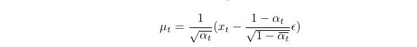

We have xₜ by adding noise ϵ t times to the base image using the forward process using
Eventually the model needs to train a noise estimator .
Training and Inference

For training, take a random timestep and train the network to predict noise level at this timestep. At inference, go through entire T iterations of model. Starting at a noisy image from the normal distribution. For timestep t > 1, an additive sampled noise from the normal distribution is added to denoised sample to form a sample. The additive noise is added to approximate the distribution of x_{t-1} and to create some diversity to the DDPM model.
Acknowledge
The blog post is based on the Paper "Denoising Diffusion Probabilistic Models" by Jonathan Ho, Ajay Jain, Pieter Abbeel at the 34th Conference of Neural Information Processing Systems 2020. arxiv paper link
Reference used in this blog post