6-1 군집 알고리즘

학습 목표

• 흑백 사진을 분류하기 위해 여러 가지 아이디어를 내면서 비지도 학습솨 군집 알고리즘에 대해 이해한다.

1) 과일 사진 데이터 확인

📕 데이터 준비

• 데이터 불러오기

fruits = np.load('fruits_300.npy')
print(fruits.shape)
▶
(300, 100, 100)

• 데이터 확인

# imshow로 numpy 배열로 저장된 이미지 출력(밝을수록 255 짙을수록 0)
plt.imshow(fruits[0], cmap='gray')
plt.show()

# cmap = 'gray_r'로 흑백을 반전(밝을수록 0 짙을수록 255)
plt.imshow(fruits[0], cmap='gray_r')
plt.show()

# 파인애플, 바나나 이미지 출력
fig,axs = plt.subplots(1,2)
axs[0].imshow(fruits[100], cmap='gray_r')
axs[1].imshow(fruits[200], cmap='gray_r')
plt.show()

• 결과 이미지

• 사과
  

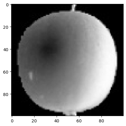
• 사과(흑백반전)
  

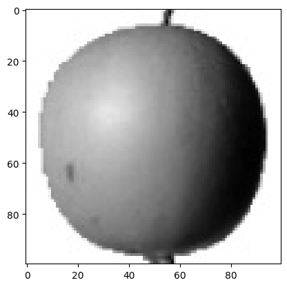
• 파인애플, 바나나
  

📕 픽셀값 분석하기

• 과일별 데이터 구분

apple = fruits[:100].reshape(-1,100*100)
pineapple = fruits[100:200].reshape(-1,100*100)
banana = fruits[200:300].reshape(-1,100*100)

apple.shape, pineapple.shape, banana.shape
▶
((100, 10000), (100, 10000), (100, 10000))

• 과일에 따른 이미지별 평균 픽셀값 확인

# 과일별 평균 픽셀값의 히스토그램
plt.hist(np.mean(apple, axis=1), alpha=0.8, label = 'apple')
plt.hist(np.mean(pineapple, axis=1), alpha=0.8, label = 'pineapple')
plt.hist(np.mean(banana, axis=1), alpha=0.8, label = 'banana')
plt.legend()
plt.show()

• 결과 이미지

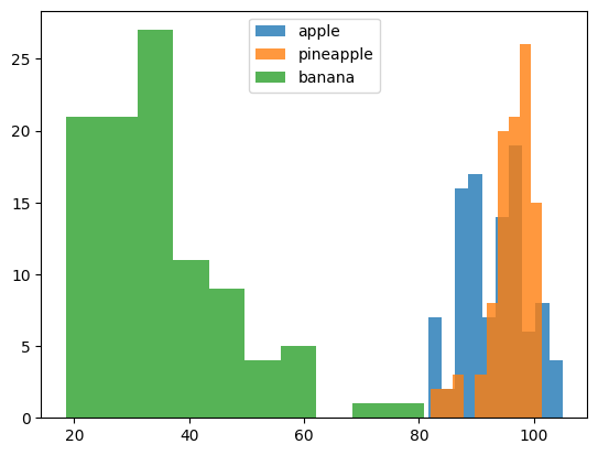
바나나 사진의 평균값은 40 아래에 집중되어 있고, 사과와 파인애플은 90~100 사이에 많이 모여 있다.
바나나는 이미지 내에서 바나나가 차지하는 영역이 작기때문에 평균값이 작다.
픽셀의 평균값으로 바나나는 구분이 가능하지만 사과나 파인애플은 구분이 힘들다.

• 과일에 따른 픽셀별 평균값 확인

fig, axs = plt.subplots(1,3,figsize=(20,5))
axs[0].bar(range(10000), np.mean(apple, axis=0))
axs[1].bar(range(10000), np.mean(pineapple, axis=0))
axs[2].bar(range(10000), np.mean(banana, axis=0))
plt.show()

• 결과 이미지
  
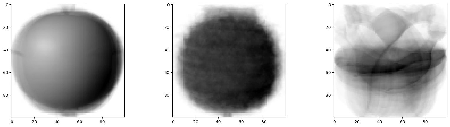
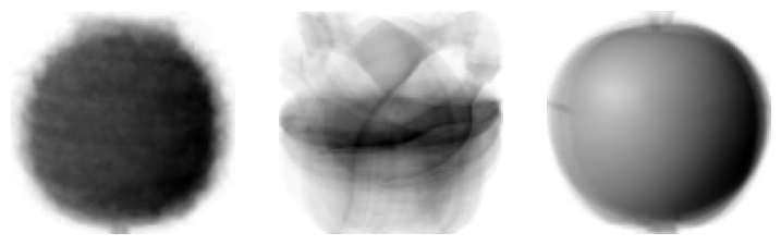
  사과는 사진 아래쪽으로 갈수록 값이 높아지고, 파인애플은 전체적으로 고르면서 높고, 바나나는 중앙의 픽셀값이 높다.

• 픽셀 평균값을 100*100 크기로 바꿔서 이미지로 출력(픽셀별 평균값으로 이미지 재생성)

apple_mean = np.mean(apple, axis=0).reshape(100,100)
pineapple_mean = np.mean(pineapple, axis=0).reshape(100,100)
banana_mean = np.mean(banana, axis=0).reshape(100,100)

fig,axs = plt.subplots(1,3,figsize=(20,5))
axs[0].imshow(apple_mean, cmap='gray_r')
axs[1].imshow(pineapple_mean, cmap='gray_r')
axs[2].imshow(banana_mean, cmap='gray_r')
plt.show()

• 결과 이미지
  

2) 평균값과 가까운 사진 고르기

📕 평균 오차 구하기

• abs_diff는 (300,100,100) 크기의 배열이다. 따라서 각 샘플에 대한 평균을 구하기 위해 axis에 두번째, 세번재 차원을 모두 지정하였다.
  이렇게 계산한 abs_mean은 각 샘플의 오차 평균이므로 크기가 (300,)인 1차원 배열이다.

abs_diff = np.abs(fruits - apple_mean)
abs_mean = np.mean(abs_diff, axis=(1,2))
print(abs_mean.shape)
▶
(300,)

📕 평균 오차가 작은 샘플 추출

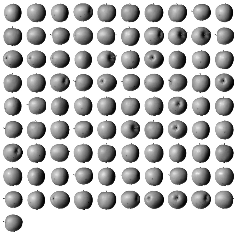
• 이 값이 가장 작은 순서대로 100개를 골라서, 즉 apple_mean과 오차가 가장 작은 샘플 100개를 뽑아보자.

apple_index = np.argsort(abs_mean)[:100]
fig, axs = plt.subplots(10,10,figsize=(10,10))
for i in range(10):
    for j in range(10):
        axs[i,j].imshow(fruits[apple_index[i*10+j]], cmap='gray_r')
        axs[i,j].axis('off') # 축을 안보이게 함
plt.show()

• 결과 이미지
  

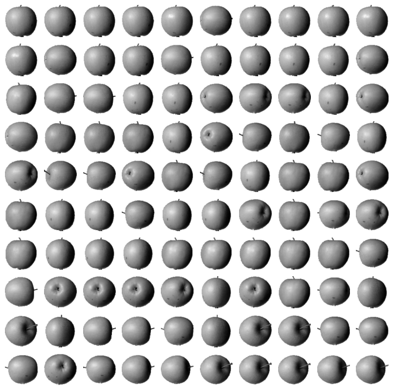
apple_mean과 가장 가까운 사진 100개가 전부 사과이다.

❗ discussion
이렇게 비슷한 샘플끼리 그룹으로 모으는 작업을 군집(clustering)이라고 한다. 군집은 대표적인 비지도 학습 작업 중 하나이며, 이 군집 알고리즘에서 만든 그룹을 클러스터라고 한다.

📕 키워드 정리

비지도 학습
머신러닝의 한 종류로 훈련 데이터에 타깃이 없고, 그로 인해 외부의 도움 없이 스스로 유용한 무언가를 학습해야함

히스토그램
구간별로 값이 발생한 빈도를 그래프로 표시한 것

군집
비슷한 샘플끼리 하나의 그룹으로 모으는 대표적인 비지도 학습 작업

6-2 k-평균

학습 목표

• k-평균 알고리즘의 작동 방식을 이해하고 과일 사진을 자동으로 모으는 비지도 학습 모델을 만들어 봅니다.

1) k-평균 알고리즘

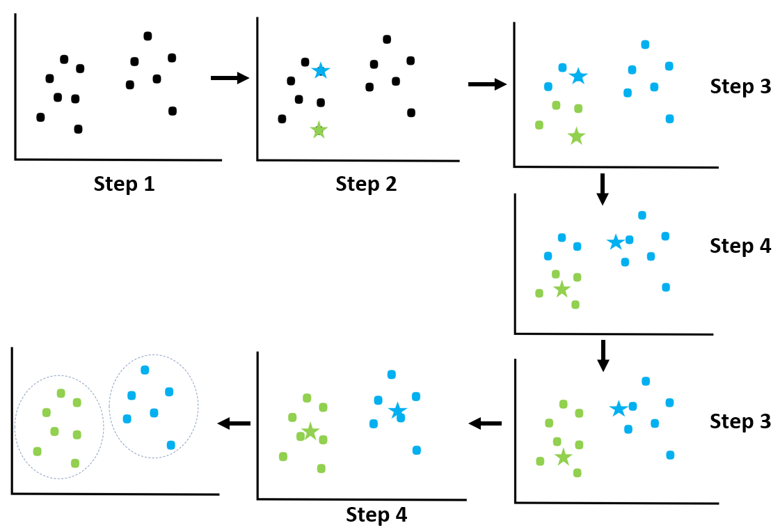
📕 k-평균 알고리즘 작동 방식

1. 무작위로 k개의 클러스터 중심을 정한다.
2. 각 샘플에서 가장 가까운 클러스터 중심을 찾아 해당 클러스터의 샘플로 지정
3. 클러스터에 속한 샘플의 평균값으로 클러스터 중심을 변경
4. 클러스터 중심에 변화가 없을 때까지 2번으로 돌아가 반복한다.

• 작동 메커니즘 도식화
  

2) scikitlearn k-means model

📕 데이터 불러오기

• fruits 데이터

import numpy as pn
fruits = np.load('fruits_300.npy')
fruits_2d = fruits.reshape(-1,100*100)

📕 scikit learn k-means

• KMeans 클래스 학습

from sklearn.cluster import KMeans
km = KMeans(n_clusters=3, random_state=42)
km.fit(fruits_2d)
print(np.unique(km.labels_, return_counts=True))
▶
(array([0, 1, 2], dtype=int32), array([111,  98,  91]))

첫번째 클러스터(레이블 0)가 111개의 샘플을 모았고, 두번째 클러스터(레이블 1)가 98개의 샘플을 모았고 세번째 클러스터(레이블 2)는 91개의 샘플을 모았다.

📕 각 클러스터에 모인 이미지 확인

• 클러스터별 이미지 생성 함수 생성

import matplotlib.pyplot as plt
def draw_fruits(arr, ratio=1) :
    n = len(arr) # n은 샘플 개수
    # 한 행에 10개씩 이미지 생성
    rows = int(np.ceil(n/10))
    # 행이 1개면 열의 개수는 샘플 개수, 그렇지 않으면 10개
    cols = n if rows < 2 else 10
    
    fig,axs = plt.subplots(rows, cols, figsize=(cols*ratio, rows*ratio), squeeze=False)
    for i in range(rows):
        for j in range(cols):
            if i*10 + j < n :
                axs[i,j].imshow(arr[i*10+j], cmap='gray_r')
            axs[i,j].axis('off')
    plt.show()

• 각 라벨별 클러스터 이미지 추출

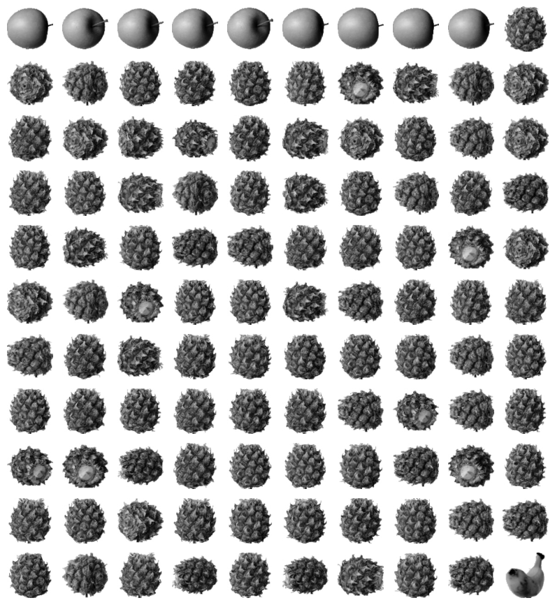
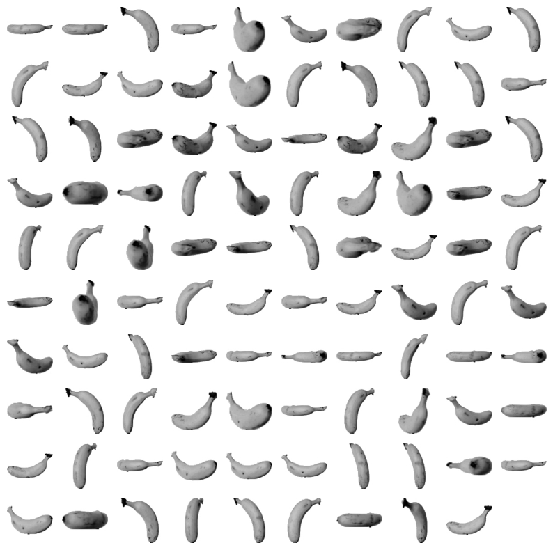
draw_fruits(fruits[km.labels_==0])
draw_fruits(fruits[km.labels_==1])
draw_fruits(fruits[km.labels_==2])

• 결과이미지

• label==0
  

• label==1
  

• label==2
  

레이블이 1인 클러스터는 바나나로만 이루어져 있으나,
레이블이 2인 클러스터는 사과 9개와 바나나 2개가 섞여있다.

• 클러스터 중심: shape이 (3,10000)이므로 리사이징 필요

draw_fruits(km.cluster_centers_.reshape(-1,100,100), ratio=3)

• 결과 이미지
  

📕 샘플에 적용하기

• 인덱스가 100인 샘플에 transform() 메서드 적용하여 새로운 클러스터 중심 찾기

print(km.transform(fruits_2d[100:101]))
▶
[[3393.8136117  8837.37750892 5267.70439881]]

• 인덱스가 100인 샘플의 레이블 예측하기
  위에서 label==0인 클러스터 중심과의 거리가 가장 가까우므로 label==0

print(km.predict(fruits_2d[100:101]))
▶
[0]

draw_fruits(fruits[100:101])

• 결과 이미지
  

• k-means 알고리즘이 반복한 횟수 확인

print(km.n_iter)
▶
4

3) 최적의 k 찾기

📕 엘보우 방법으로 최적의 k 찾기

• 클러스터 중심과의 거리 제곱합인 inertia를 클러스터 개수를 증가시키면서 확인해보자. inertia의 기울기가 완만해지는 지점이 최적의 k이다.

inertia= []
for k in range(2,7) :
    km = KMeans(n_clusters=k, random_state=42)
    km.fit(fruits_2d)
    inertia.append(km.inertia_)
plt.plot(range(2,7), inertia)
plt.xlabel('k')
plt.ylabel('inertia')
plt.show()

📕 키워드 정리

k-means
랜덤한 초기값을 가진 클러스터의 중심을 정하고, 이동&재설정을 반복하여 최적의 클러스터를 구성하는 알고리즘

클러스터 중심(centroid)
k-means 알고리즘이 만든 클러스터에 속한 샘플의 특성 평균값

엘보우 방법
최적의 클러스터 개수를 정하는 방법 중 하나이다. 클러스터 중심과 샘플 사이 거리의 제곱 합을 이너셔라고 하는데, 클러스터 개수에 따라 이너셔 감소가 꺾이는 지점이 적절한 클러스터 개수 k가 될 수 있다.

6-3 주성분 분석

학습 목표

• 차원 축소에 대해 이해하고, 대표적인 차원 축소 알고리즘 중 하나인 PCA(주성분 분석) 모델을 만들어 본다.

1) 주성분 분석 소개

📕 PCA 클래스

from sklearn.decomposition import PCA
pca = PCA(n_components=50)
pca.fit(fruits_2d)
print(pca.components_.shape)
▶
(50, 10000)

draw_fruits(pca.components_.reshape(-1,100,100))

• 결과 이미지
  
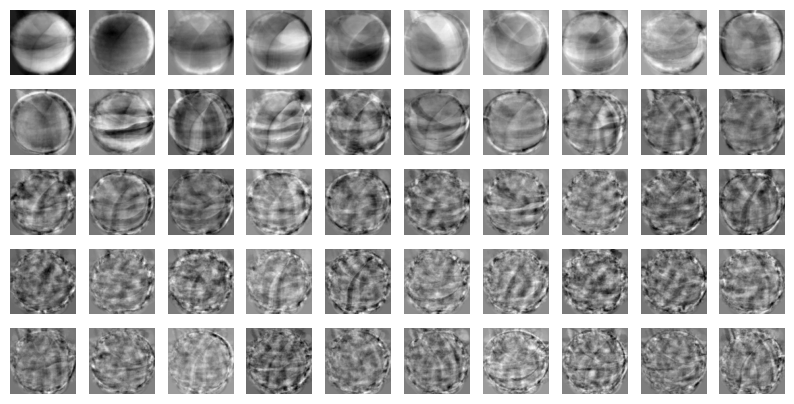
  이 주성분은 원본 데이터에서 가장 분산이 큰 방향을 순서대로 나타낸 것이다.

📕 원본 데이터 차원 축소

• 원본 데이터의 차원을 10000에서 50으로 축소

print(fruits_2d.shape)
▶
(300, 10000)

fruits_pca = pca.transform(fruits_2d)
print(fruits_pca.shape)
▶
(300, 50)

2) 원본 데이터 재구성

📕 원본 데이터 특성 복원

fruits_inverse = pca.inverse_transform(fruits_pca)
print(fruits_inverse.shape)
▶
(300, 10000)

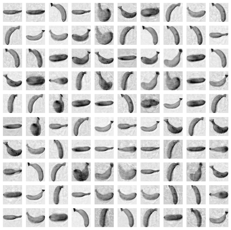
fruits_reconstruct = fruits_inverse.reshape(-1,100,100)
for start in [0,100,200]:
    draw_fruits(fruits_reconstruct[start:start+100])
    print('\n')

• 결과 이미지
  
  
  

3) 설명된 분산

📕 분산 비율의 합

• 주성분이 원본 데이터의 분산을 얼마나 잘 나타내는지 기록한 값을 설명된 분산(explained variance)라고 한다. PCA 클래스의 explainedvariance_ratio에 각 주성분의 설명된 분산 비율이 기록되어 있다. 이들의 합을 통해 추출한 주성분으로 표현하고 있는 총 분산 비율을 얻을 수 있다.

print(np.sum(pca.explained_variance_ratio_))
▶
0.9215956549690777

plt.plot(pca.explained_variance_ratio_)
plt.show()

• 결과 이미지
  

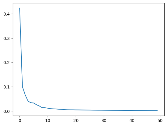
처음 10개의 주성분이 상위의 분산비율을 가지고, 그 이후로는 각 주성분이 설명하고 있는 분산은 비교적 작다.

4) 다른 알고리즘과 함께 사용하기

과일 사진 원본 데이터와 PCA로 축소한 데이터를 지도 학습에 적용해보고 어떤 차이가 있는지 알아보자.

📕 로지스틱 회귀 함수 활용

• 함수 및 target 생성

from sklearn.linear_model import LogisticRegression
lr = LogisticRegression()

# 사과, 파인애플, 바나나 순서대로 0,1,2로 라벨 지정
target = np.array([0]*100 + [1]*100 + [2]*100)

• 원본 데이터 성능 확인

from sklearn.model_selection import cross_validate
scores = cross_validate(lr, fruits_2d, target)
print(np.mean(scores['test_score']))
print(np.mean(scores['fit_time']))
▶
0.9966666666666667
1.7810904026031493

• 주성분 분석으로 축소한 데이터 성능 확인

from sklearn.model_selection import cross_validate
scores = cross_validate(lr, fruits_pca, target)
print(np.mean(scores['test_score']))
print(np.mean(scores['fit_time']))
▶
1.0
0.020934200286865233

50개의 특성만 사용했는데도 정확도가 100%이고, 훈련 시간은 0.03초로 20배 이상 감소하였다.

📕 설명된 분산의 비율로 주성분 개수 확인

• n_components 매개변수에 원하는 설명된 분산의 비율을 입력할 수 있다.

pca = PCA(n_components=0.5)
pca.fit(fruits_2d)
print(pca.n_components_)
▶
2

단 2개의 특성만으로 원본 데이터에 있는 분산의 50%를 표현할 수 있다.

• 주성분 2개인 데이터로 훈련한 모델 성능 확인

fruits_pca = pca.transform(fruits_2d)
print(fruits_pca.shape)
▶
(300, 2)

scores = cross_validate(lr, fruits_pca, target)
print(np.mean(scores['test_score']))
print(np.mean(scores['fit_time']))
▶
0.9933333333333334
0.039040756225585935

2개의 특성만 사용해도 99%의 정확도를 달성하였다.

📕 차원 축소된 데이터로 클러스터 확인

from sklearn.cluster import KMeans
km = KMeans(n_clusters=3, random_state=42)
km.fit(fruits_pca)
print(np.unique(km.labels_, return_counts=True))
▶
(array([0, 1, 2], dtype=int32), array([110,  99,  91]))

for label in range(0,3):
    draw_fruits(fruits[km.labels_==label])
    print('\n')

• 결과이미지

• label==0
  

• label==1
  

• label==2
  

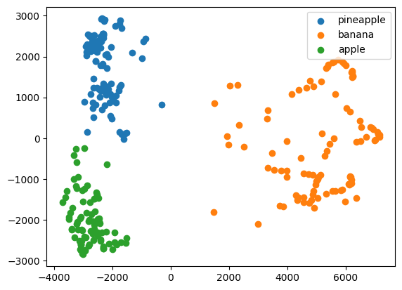
원본 데이터로 찾은 클러스터와 비슷하게 파인애플과 사과가 조금 혼돈되는 면이 있다.

• 시각화 : 2차원으로 줄였기에 2차원 시각화가 가능하다.

for label in range(0,3) :
    data = fruits_pca[km.labels_ == label]
    plt.scatter(data[:,0], data[:,1])
plt.legend(['pineapple','banana','apple'])
plt.show()

• 결과 이미지
  

📕 키워드 정리

차원 축소
원본 데이터의 특성을 적은 수의 새로운 특성으로 변환하는 비지도 학습의 한 종류

주성분 분석
차원 축소 알고리즘의 하나로 데이터에서 가장 분산이 큰 방향을 찾는 방법이다. 이런 방향을 주성분이라고 하며, 원본 데이터를 주성분에 투영하여 새로운 특성을 만들 수 있다. 일반적으로 주성분은 원본 데이터에 있는 특성 개수보다 작다.

설명된 분산
주성분 분석에서 주성분이 얼마나 원본 데이터의 분산을 잘 나타내는지 기록한 것