[머신러닝 교과서] 파이썬 그래프 그리기

장채민·2024년 12월 30일

퍼셉트론 클래스

Perceptron ( eta=0.1 , n_iter=10 , random_state=1 )

eta: 학습률
//퍼셉트론에서 가중치를 업데이트할 때, 얼마나 큰 폭으로 조정할지를 결정하는 값
//값이 작을수록 천천히 학습하고, 값이 클수록 빠르게 학습함
//값을 너무 작게 설정하면 학습이 오래 걸리고, 너무 크면 학습이 불안정해질 수 있음
//0.0과 1.0 사이

n_iter: 훈련 데이터셋 반복 횟수
//데이터셋 전체를 몇번 반복해서 학습할지를 나타냄
//데이터셋 크기와 복잡성에 따라 적절한 값을 설정해야함
//보통 10~100 사이의 값을 많이 사용함

random_state: 가중치 무작위 초기화를 위한 난수 생성 시드
//가중치, 학습 데이터의 처리 순서에 사용되는 난수를 고정시켜 실험 조건을 동일하게 유지시킴
//난수 생성기가 동일한 시드 값을 가지면 동일한 난수를 생성함
//시드 값의 크기는 가중치의 초기값 등에 영향을 주지 않으며 난수 생성의 패턴만 고정하는 역할을 함
//관례적으로 random_state=42가 많이 사용되기는 함. 하지만 다른 숫자여도 크게 상관없음


import numpy as np

class perceptron:

   // 객체 생성 시 호출되는 생성자(constructor)로 초기화 또는 기본값 설정해줌
   def __init__(self, eta=0.01, n_iter=50, random_state=1): //매개변수
      self.eta=eta
      self.n_iter=n_iter
      self.random_state=random_state
      
   def fit(self, X, y):
      # X:학습데이터(특징 행렬, 샘플개수X특징개수)
      # y:학습데이터의 레이블(타깃 값)
      
      //난수 생성하는 객체
      rgen=np.random.RandomState(self.random_state)
      
      //가중치 벡터 w를 정규분포 난수(0에 가까운 수)로 초기화
      self.w_=rgen.normal(loc=0.0, scale=0.01, size=X.shape[1])   
      #rgen.normal은 정규분포로 난수 생성하는 함수
      #loc=0.0: 정규분포의 평균값을 0으로 설정
      #scale=0.01: 표준편차를 0.01로 설정
      #size=X.shape[1]: 난수의 개수를 X의 특징 개수만큼 생성
      
      //절편 0으로 초기화
      self.b_=np.float64(0.0)
      
      //에러 횟수 저장할 리스트
      self.errors_=[]     
      
      for _ in range(self.n_iter):   //에포크 수(학습의 반복 횟수)만큼 반복
         errors=0    //error 변수는 0으로 초기화
         for xi, target in zip(X,y):   //내부 루프
            update=self.eta*(target-self.predict(xi))  
            //변수 update는 학습률*오차 로 계산
            self.w_+=update*xi     //가중치 업데이트
            self.b_+=update       //절편 업데이트
            errors+=int(update!=0.0)     //잘못된 예측 횟수 저장
            # int(boolean값): true이면() 1 반환, false이면 0 반환
         self.errors_.append(errors)    //에포크별 오류 기록
      return self
      
   def net_input(self,X):
      return np.dot(X,self.w_) + self.b_   
      // 선형 결합 계산
      // np.dot은 행렬 곱을 수행해 x와 가중치w의 내적을 계산함
      // 결과: 1차원 배열(각 샘플의 출력값)
      
   def predict(self,X):
      return np.where(self.net_input(X) >= 0.0, 1, 0)
      //단위 계단 함수를 사용하여 클래스 레이블 반환
      //np.where(조건, 참인 경우 반환값, 거짓인 경우 반환값)

matplotlib을 이용한 Iris 꽃의 산점도 그리기

matplotlib.pyplot: 데이터 시각화를 위한 라이브러리

import os
import pandas as pd
import matplotlib.pyplot as plt
import numpy as np

s='https://archive.ics.uci.edu/ml/machine-learning-databases/iris/iris.data'
print('URL:',s)

df=pd.read_csv(s,header=None,encoding='utf-8')
// url에서 Iris 데이터셋을 CSV 형식으로 읽어옴
// header=None: 데이터에 컬럼 이름이 없으므로 자동으로 숫자 인덱스 사용하기
// encoding='utf-8': 데이터의 문자 인코딩 지정
print(df.tail())
//데이터프레임의 마지막 5개 행 출력하기


//종속 변수(y)와 독립 변수(X) 정의

y=df.iloc[0:100,4].values
//0행부터 99행, 4열의 데이터 선택 + values 이용해 numpy ndarray로 변환
y=np.where(y=='Iris-setosa',0,1)
//Iris-setosa이면 0 반환, 그렇지 않으면 1 반환

X=df.iloc[0:100,[0,2]].values
//0행부터 99행, 0열과 2열의 데이터 선택 + values 이용해 numpy ndarray로 변환
//100개의 샘플과 두개의 특징으로 구성된 2차원 배열


// 산점도(Scatter plot) 그리기
// matplotlib.pyplot 모듈의 scatter() 함수 이용
plt.scatter(X[:50,0], X[:50,1],
            color='red',marker='o',label='Setosa')
# Setosa: 빨간색 원 (o)
           
plt.scatter(X[50:100,0], X[50:100,1],
            color='blue',marker='s',label='Versicolor')
# Versicolor: 파란색 사각형 (s)            

plt.xlabel('Sepal length [cm]')
plt.ylabel('Petal length [cm]')

// 범례 그리기 (위치: 그래프의 왼쪽 위)
plt.legend(loc='upper left')

// 그래프 화면에 출력하기
plt.show()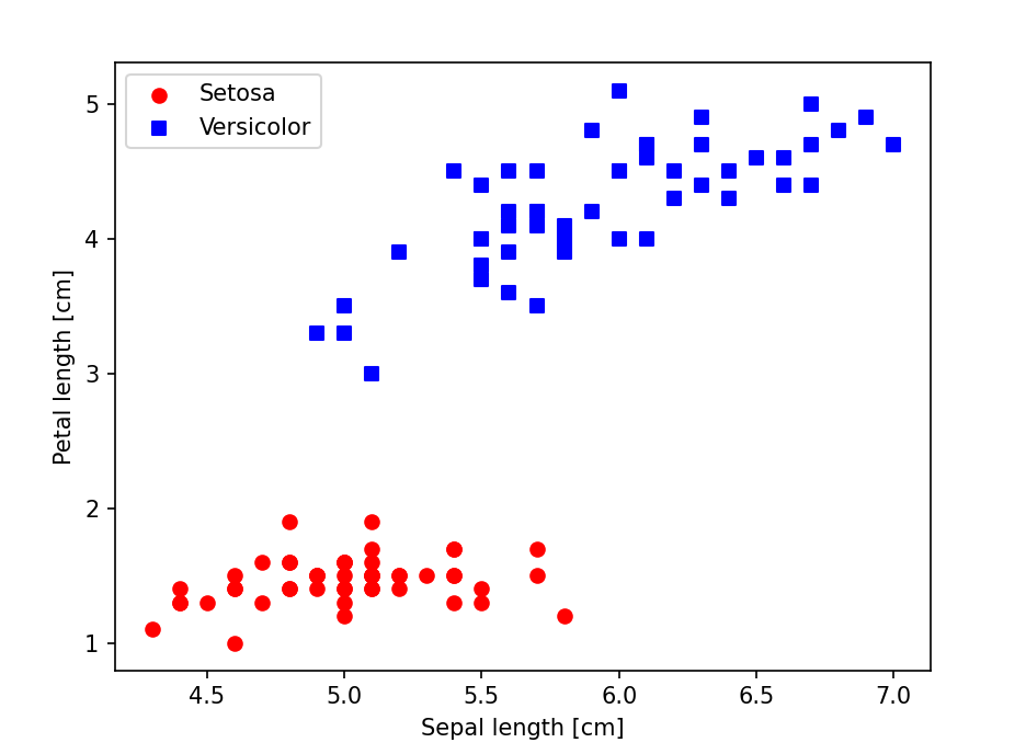

에포크 대비 잘못 분류된 오차 그래프 그리기

plt.plot(x,y)

ppn=Perceptron(eta=1,n_iter=10)
ppn.fit(X,y)

plt.plot(range(1,len(ppn.errors_)+1),ppn.errors_, marker='o')

plt.xlabel('Epochs')
plt.ylabel('Number of updates')

plt.show()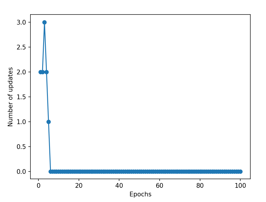

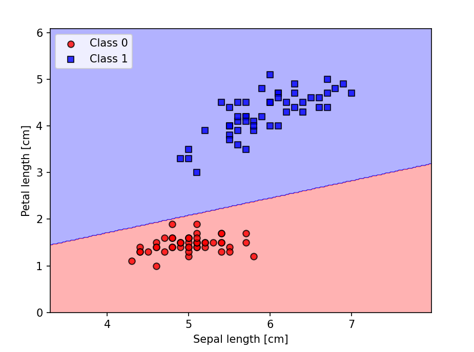
퍼셉트론이 만든 붓꽃 데이터셋의 결정 경계

def plot_decision_regions(X,y,classifier,resolution=0.02):
    markers=('o','s','^','v','<')
    colors=('red','blue','lightgreen','gray','cyan')
    //튜플로 점의 모양과 색상 정의
    cmap=ListedColormap(colors[:len(np.unique(y))])
    //y는 [0,1]로 두개의 클래스만 존재
    //colors에서 red와 blue만 사용
    //matplotlib의 colors 객체
    //cmap.colors 출력하면 ('red','blue') 나옴
    
    x1_min, x1_max=X[:,0].min()-1, X[:,0].max()+1
    x2_min, x2_max=X[:,1].min()-1, X[:,1].max()+1
    
    xx1, xx2=np.meshgrid(np.arange(x1_min, x1_max, resolution),
                         np.arange(x2_min, x2_max, resolution))
    // 직사각형 그리드 생성  
                       
    lab=classifier.predict(np.array([xx1.ravel(),xx2.ravel()]).T)
    // .T (Transpose) 는 배열을 전치하여 행과 열을 뒤바꾼다
    
    lab=lab.reshape(xx1.shape)
    plt.contourf(xx1,xx2,lab,alpha=0.3,cmap=cmap)
    plt.xlim(xx1.min(),xx1.max())
    plt.ylim(xx2.min(),xx2.max())
    
    for idx, cl in enumerate(np.unique(y)):
        plt.scatter(x=X[y==cl,0],
                    y=X[y==cl,1],
                    alpha=0.8,
                    c=colors[idx],
                    marker=markers[idx],
                    label=f'Class {cl}',
                    edgecolor='black')


ppn=Perceptron(eta=1,n_iter=10)
ppn.fit(X,y)

plot_decision_regions(X,y,classifier=ppn)
plt.xlabel('Sepal length [cm]')
plt.ylabel('Petal length [cm]')
plt.legend(loc='upper left')
plt.show()