[논문리뷰] CALF: Aligning LLMs for Time Series Forecasting via Cross-modal Fine-Tuning

Oliver·2025년 1월 17일

Arxiv link

Github page

Introduction

Multivariate time series forecasting (MTSF)는 time series analysis에서 중요한 역할을 하며, single modality에 기반한 DL based Method들이 개발되어 왔다. 그러나 이런 single modal MTSF method들은 제한된 training data로 인해 overfitting 문제로부터 자유롭지 못하다. 이러한 issue들을 해결하기 위해 일부 연구들은 LLM의 context modeling ability를 사용하여 MTSF를 수행하고자 하였다. Large-scale의 pre-training을 이용하여 LLM은 context modeling 능력을 보여줄 뿐 아니라 overfitting 문제도 해결할 수 있다.

기존의 LLM을 이용하여 MTSF를 수행하는 작업은 LLM을 adapting하고 fine-tuning하는데에만 집중하였다. 이 과정에서 textual input token과 temporal input token간의 distribution discrepancy를 간과하여 최적의 성능을 달성하는데 실패하는 경우가 많았다. 실제로 최근의 LLM based method들은 pre-trained LLM을 목적에 맞게 well initialized된 forecasting model로 취급하며, linear layer에 input time series를 projection하여 LLM의 입력으로 넣는다. 이는 직관적이긴 하나 distribution discrepancy를 간과한다는 문제가 있다.

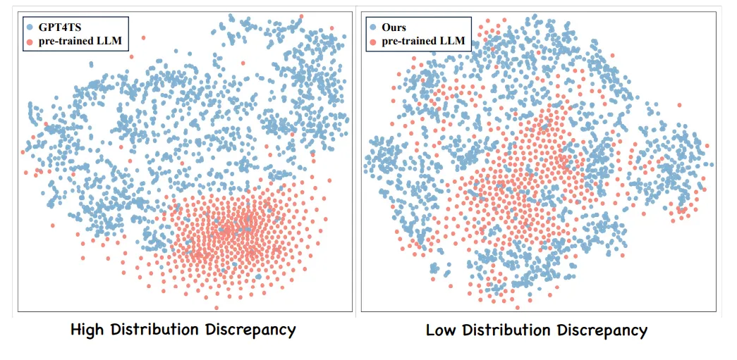
t-SNE visualization or pre-trained word token dmbeddings of LLM. 
GPT4TS라고 불리는 LLM based MTSF에서는 textual token과 temporal token의 분포가
잘 맞지 않는 것을 확인할 수 있다.
이 연구의 경우 분포가 나름 잘 분산되어 있는 것을 볼 수 있다.

이 연구는 Cross-ModAl LLM Fine-Tuning (CALF) framework를 제안한다. 여기서는 cross-modal fine-tuning을 이용하여 temporal target modalities와 textual source modalities를 comprehensive 하게 alignment할 수 있도록 한다.

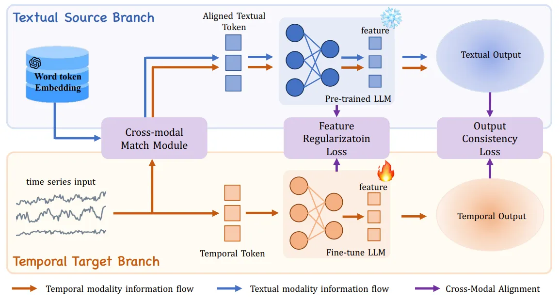
구체적으로 CALF는 2가지 구성요소로 나뉜다 : temporal target branch와 textual source branch이다. temporal target branch는 time seires information을 리하며, textual source branch는 textual modal token을 이용해 pre-trained된 LLM의 information을 추출하고 time series에 맞게 적응시킨다. 이 두 branch간의 modality gap을 해소하기 위해 3가지의 cross-modal fine-tuning techniques을 도입한다.

Cross-Modal Match Module: principle word embedding extraction과 cross-attention mechanism을 이용해 time series - textual input을 통합한다. 이를 통해 time series와 text간의 marginal input distribution을 align할 수 있다.
Feature Regularization Loss: 각 intermediate layer의 output을 aligns하여 gradient를 계산하도 weight update에 도움을 준다.
Output Consistency Loss: textual and temporal series modality가 효과적으로 대응됙 ㄹ 수 있도록 하며, representation space에서 discrepancies를 해결하고 time series data의 semantic context를 유지한다.

Method

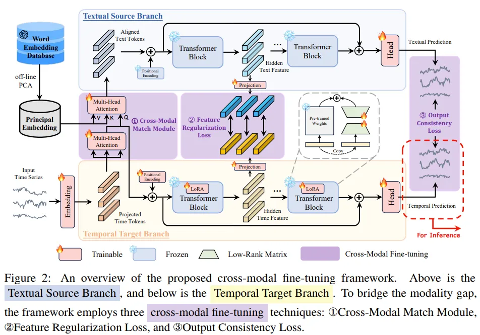
Textual source branch는 aligned text token $X_{text}$ 를 input으로 받으며, Pre-trained LLM layer $L$ 개를 이용하여 hidden text feature $F_{text}^l, l = \{1, ..., L\}$ 을 얻는다. 이후 task-specific head를 이용해 output $Y_{text}$ 를 얻는다. temporal target branch는 projected된 time series token $X_{time}$ 을 받으며, textual source branch에서와 같은 LLM layer $L$ 개를 이용해 hidden time feature $F_{time}^l$ 을 얻는다. 이 branch에서 나오는 출력은 $Y_{time}$ 로 표기하기로 한다.

두 branch의 modality gap을 해소하기 위해, Cross-Modal Match Module, Feature Regularization Loss, Output Consistency Loss을 이용한다.

1. Cross-Modal Match Module

Pre-trained LLM의 matrics of word embedding layer은 context representation space를 형성하여 단어 간의 의미적 거리를 vector similarity를 통해 정량화할 수 있다. 이 word embedding layer는 pre-trained LLM에서 language modality의 distribution을 나타낸다. 기존 방법들은 이러한 distribution을 무시하고 time series data를 projection하여 LM의 input dimension에 맞게 한다.

이 연구에서는 time series의 distribution을 LLM의 word embedding과 align하는 방법으로 Cross-Modal Match Module을 제안한다. Multivariate time series $I \in \mathbb{R}^{T \times C}$ (T: input sequence length, C: # of variants) 일 때 embedding layer과 Multi-Head Self Attention을 이용해 projected time tokens $X_{time}$ 을 얻는다.

X_{time} = MHSA(Embedding(I)) \in \mathbb{R}^{C \times M}

M은 pre-trained된 LLM의 feature dimension이다. Embedding layer $Embedding(.)$ 은 $T$ 에서 $M$ 으로의 channel-wise dimensional mapping을 수행한다.

이후 $X_{time}$ 을 temporal modality로, word embedding dictionaries $\mathcal{D} \in \mathbb{R}^{|\mathcal{A}| \times M}$ ( $|\mathcal{A}|$ : size of alphabet)을 textual modality로 align하기 위해 cross-attention을 적용한다. $|\mathcal{A}|$ 의 크기가 GPT2의 경우 50257일 정도로 매우 커서 직접 사용하기에는 게산 비용이 높아진다는 문제가 있다. 이를 해결하기 위해 의미적으로 비슷한 단어들은 “synonym cluster”을 형성한다는 점을 이용해 주변 단어들을 cluster center을 이용해 표현하는 word embedding extraction 전략을 제안한다. 구체적으로는 PCA를 사용하여 $\mathcal{D}$ 의 차원을 축소하여 principal word embedding $\mathcal{\hat{D}} \in \mathbb{R}^{d \times M}$ 을 얻는다.

\mathcal{\hat{D}} = PCA(\mathcal{D})

여기서 d는 pre-defined된 low dimension이며 $d \ll |\mathcal{A}|$ 를 만족한다. 이 과정은 학습 전 1번만 수행된다.

이후 $\mathcal{\hat{D}}$ 를 Key / Value로, $X_{time}$ 을 Query로 사용하여 Multi-head Cross-Attention을 수행하여 principal word embedding과 temporal token을 align하여 aligned text token $X_{text} \in \mathbb{R}^{C \times M}$ 을 얻는다.

X_{text} = Softmax(\frac{QK^T}{\sqrt{C}})V, \\Q = X_{time}W_q, K = \mathcal{\hat{D}}W_k, V = \mathcal{\hat{D}}W_v

여기서 $W_q, W_k, W_v \in \mathbb{R}^{M \times M}$ 은 Q, K, V의 projection matrix이다.

2. Feature Regularization Loss

LLM의 Pre-trained weight는 textual modality data에 기반한다. 이를 time series data에 adapt시키기 위해 temporal target branch의 각 layer의 output을 textual source branch의 출력과 align하는 과정이 필요하다. 이는 Feature Regularization Loss에 의해 이루어지며 두 branch의 intermediate feature을 일치시켜 각 중간 레이어들의 gradient를 효과적으로 계산하고 가중치를 업데이트 할 수 있도록 돕는다. 구체적으로 textual source branch와 temporal target branch의 l번째 transformer block의 output $F_{text}^l, F_{time}^l$ 이 주어졌을 때 다음과 같이 정의할 수 있다.

\mathcal{L}_{feature} = \sum^L_{i = 1} \gamma ^{L-i}sim(\phi^{text}_i(F^l_{text}), \phi^{time}_i(F^l_{time}))

$\gamma$ 는 각 layer의 loss scale을 조정하는 하이퍼파라미터, $sim(\cdot,\cdot)$ 은 L1 loss와 비슷한 similarity function이다. 또한 $\phi_l^{text}(\cdot),\phi_l^{time}(\cdot)$ 은 projection layer으로, textual / time modality의 feature들을 shared representation space로 변환한다.

3. Output Consistency Loss

위의 단계에 기반하여 여기서는 textual and temporal modality간의 semantic context를 일관성 있게 유지한다. output consistency loss는 output distribution이 효과적으로 대응될 수 있게 하여 representation space의 discrepancy를 해결한다. text source branch와 temporal target branch의 output $Y_{text}, Y_{time}$ 이 주어졌을 때 다음과 같이 정의할 수 있다.

\mathcal{L}_{output} = sim(Y_{text},Y_{time})

4. Parameter Efficient Training

catastrophic forgetting을 방지하고 학습 효율을 개선하기 위해 LLM을 fine tuning하는 과정에서 Parameter Efficient Training을 사용한다. Temporal target branch에서는 Low-rank Adaptation (LoRA)를 사용하고 positional encoding weight를 fine tuning한다. 학습의 total loss는 다음과 같다.

\mathcal{L}_{total} = \mathcal{L}_{sup} + \lambda_1\mathcal{L}_{feature} + \lambda_2\mathcal{L}_{output}

$\mathcal{L}_{sup}$ 은 supervised loss이며, $\lambda_1, \lambda_2$ 는 하이퍼파라미터이다.

Inference 단게에서는 temporal target branch의 output이 모델 전체의 output으로 간주된다.

Experiments

Baseline

Time series forecasting task를 수행하는 모델들을 카테고리에 따라 선별하였음.

LLM-based model: TimeLLM, GPT4TS
Transformer-based model: PatchTST, iTransformer, Crossformer, ETSformer,
FEDformer, Autoformer
CNN-based model: TCN, MICN, Times-Net
MLP-based model: DLinear, TiDE

shot-term forecasting을 위해 N-HiTS와 N-BEATS도 포함함

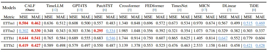
Long-term Forecasting

Electricity Transformer Temperature에서 4가지 (ETTh1, ETTh2, ETTm1, ETTm2), Weather, Electricity, Traffic dataset에 대해 실험을 진행하였다. input length는 96이며, prediction length $H \in \{96, 192, 336, 720\}$ 으로 설정하였다. Red가 best performance, Blue가 second performance이다.

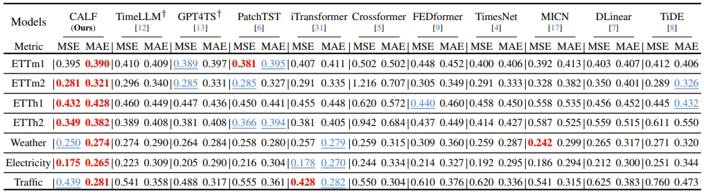
56개의 evaluation에서 좋은 성능을 달성하였다. Transformer based model인 PatchTST와 비교했을 때 MSE/MAE가 7.05%, 6.53% 감소, GPT4TS와 비교 시 5.94%, 5.14% 감소했다.

Short-term Forecasting

여기서는 M4 dataset을 사용했으며, yearly, quarterly, monthly 단위로 수집된 univariate 마케팅 데이터이다. prediction length $H \in [6, 48]$ 으로 설정되었고, input length는 prediction length의 2배로 설정된다. 평가 지표로는 symmetric mean absolute percentage error (SMAPE), mean absolute scaled error (MSAE), 그리고 overall weighted average (OWA)를 사용한다.

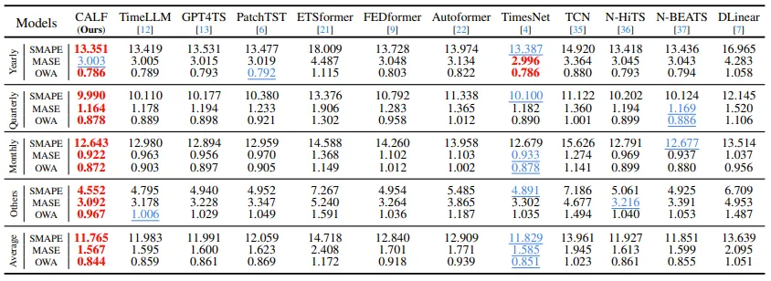
15개의 test 중 14개에서 최고 성능을 달성하였고, TimesNet과 비교 시 1%의 성능 향상이 관찰됨

Few/zero-shot Learning

Few shot learning: ETT dataset 4개에 대해 실험을 진행하였다. 각 dataset에 대해 training data의 10%만 사용하여 제한된 정보에서 학습하는 능력을 평가하였다.

GPT4TS와 PatchTST보다 각각 8%, 9% 좋은 성능을 냄
Zero shot learning: 한 dataset에서 training된 모델을 fine tuning하는 과정 없이 다른 dataset에서 테스트하는 zero-shot도 수행함.

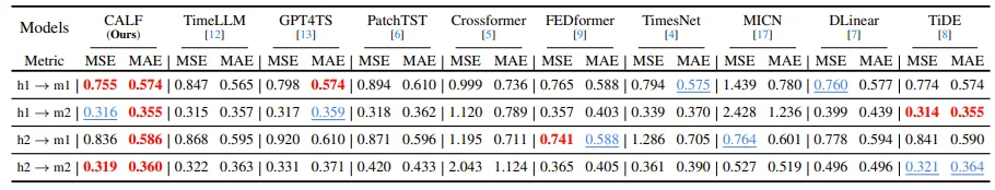
GPT4TS와 PatchTST의 성능을 각각 4%, 9% 초과하여 수행됨

Efficiency Analysis

ETTm1, ETTh1, ECL, Traffic, Weather dataset에서 실험을 수행하고, input length / prediction length는 96으로 설정하였다.

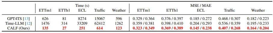
정확성과 효율성 측면에서 다른 방법들보다 상당한 개선을 보였음

Abaltion Study

Ablation on Different Loss Functions

Feature regularization loss $\mathcal{L}_{feature}$ 은 textual source branch와 temporal target branch 사이의 intermediate feature을 align하며, output consistency loss $\mathcal{L}_{output}$ 은 modality간의 output coherence를 보장한다. supervised loss $\mathcal{L}_{sup}$ 는 GT data와 함께 학습의 방향을 결정한다.

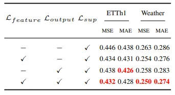
$\mathcal{L}_{feature}$ 와 $\mathcal{L}_{output}$ 을 추가하였을 때 성능의 향상이 나타나는 것을 확인할 수 있다.

Ablation on the Number of Principal Components

이 논문에서는 word embedding에 PCA를 이용하여 training cost를 절감하였는데, PCA의 경우 information loss가 발생한다는 문제점이 있다. 따라서 principal component d에 따른 효과를 분석하였다.

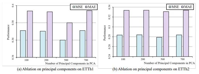
d에 따른 성능의 민감도는 그리 크지 않았으나, 너무 작은 d의 경우 key information을 놓쳐 성능 저하가 일어나고, 너무 큰 d의 경우 information redundancy가 일어나 학습 난이도가 올라간다. 본 연구에서는 d = 500을 사용하였다.

Oliver

Life of Oliver

이전 포스트

[논문리뷰] Time LLM - Time Series Forecasting by reprogramming large language model

다음 포스트