[ML] 방 분류 모델 만들기

Nicky·2024년 2월 28일

[A1BnB] AI 기반 숙소 등록 웹 서비스

목록 보기

2/14

오늘은 이용자가 등록한 사진의 방 분류를 도와줄 딥러닝 모델을 만드는 방법을 다뤄보겠다.

학습 데이터 준비

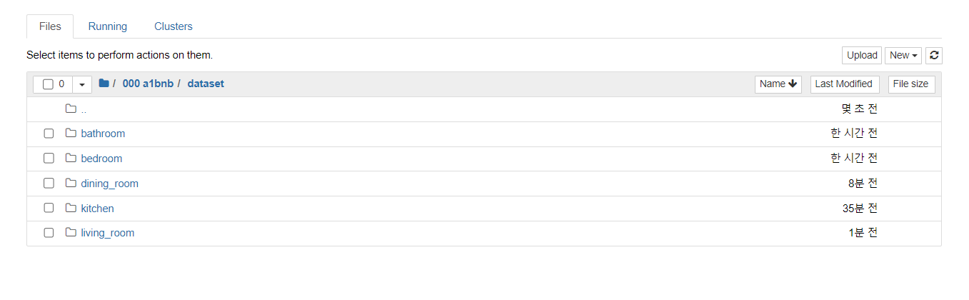
우선 모델의 학습을 위한 충분한 데이터 모델을 준비해놓아야 한다. 나의 경우 Bathroom, Bedroom, Dining_room, kitchen, Living_room 총 5가지의 클래스로 분류하기 위해 5개의 디렉토리를 생성해놓았다.

이미지 데이터셋으로는 COCO, ImageNet 등이 많이 사용된다.

모델 학습

학습은 이후 AWS Lambda에서 사용하기 좋은 경량화되고 효율적인 모델로서 MobileNet과 EfficientNetLite를 선택해 진행하였다.

import tensorflow as tf
from tensorflow.keras import layers, models, optimizers
from tensorflow.keras.preprocessing.image import ImageDataGenerator
import os

# 데이터 로드
directory = os.path.join(os.getcwd(), 'dataset/')
image_size = (224, 224)
batch_size = 32

datagen = ImageDataGenerator(
    rescale=1./255,
    validation_split=0.2)  # validation set을 위해 20% 데이터를 분할

train_generator = datagen.flow_from_directory(
    directory,
    target_size=image_size,
    batch_size=batch_size,
    class_mode='categorical',
    subset='training')  # train 데이터 설정

validation_generator = datagen.flow_from_directory(
    directory,
    target_size=image_size,
    batch_size=batch_size,
    class_mode='categorical',
    subset='validation')  # validation 데이터 설정

# 모델 불러오기
base_model = tf.keras.applications.MobileNetV2(input_shape=(224,224,3), include_top=False, weights='imagenet')
base_model.trainable = False

model = tf.keras.Sequential([
  base_model,
  layers.GlobalAveragePooling2D(),
  layers.Dense(5, activation='softmax')  # 5개 클래스에 대한 분류
])

# 손실함수, 최적화함수 설정
model.compile(optimizer=tf.keras.optimizers.SGD(lr=0.001, momentum=0.9),
              loss='categorical_crossentropy',
              metrics=['accuracy'])

# 학습
history = model.fit(train_generator, 
                    epochs=10,
                    validation_data=validation_generator)

# 모델 가중치 저장
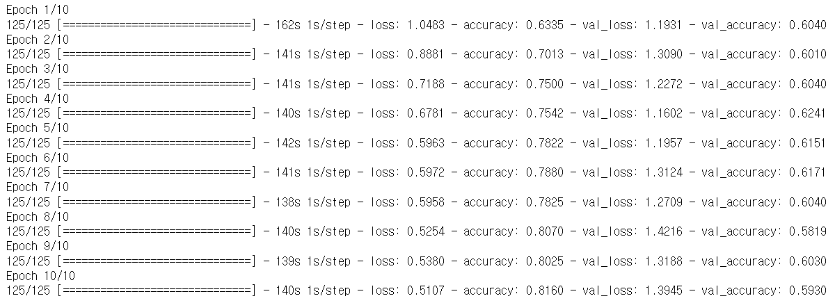
model.save_weights('model_weights.h5')

같은 환경에서 2가지 모델의 학습을 실시했을 때 결과는 다음과 같다.

MobileNetV2

loss: 0.5107, accuracy: 0.8160

EfficientNetLite

loss: 0.4736, accuracy: 0.8317

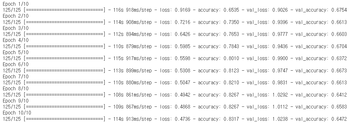
손실, 정확도는 EfficientNetLite 모델이 MobileNetV2 모델보다 더 우수하게 나왔다.

모델 추론

import tensorflow as tf
from tensorflow.keras import layers
from tensorflow.keras.preprocessing.image import load_img, img_to_array

# 모델 불러오기
base_model = tf.keras.applications.MobileNetV2(input_shape=(224,224,3), include_top=False, weights=None)
base_model.trainable = False

model = tf.keras.Sequential([
  base_model,
  layers.GlobalAveragePooling2D(),
  layers.Dense(5, activation='softmax')  # 5개 클래스에 대한 분류
])

# 모델 가중치 불러오기
model.load_weights('MobileNetV2.h5')

# 예측할 이미지 불러오기
# 여기서는 예시로 하나의 이미지를 불러옵니다. 실제로는 여러분의 이미지 경로를 사용하세요.
img = load_img('bedroom.jpg', target_size=(224, 224))

# 이미지를 모델이 처리할 수 있는 형태로 변환
img_array = img_to_array(img)
img_array = img_array / 255.0  # 이미지를 [0, 1] 범위로 스케일링
img_array = tf.expand_dims(img_array, 0)  # 배치 차원을 추가

# 이미지를 모델에 전달하여 추론
predictions = model.predict(img_array)

# 예측 결과 출력
print(predictions)

각각의 모델에 bedroom 이미지를 입력해 추론을 진행해보자.
인덱스에 따른 클래스는 다음과 같다.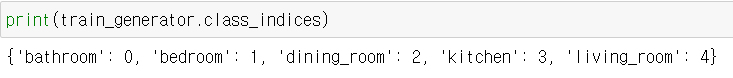

MobileNetV2

EfficientNetLite

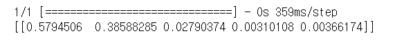
결과 비교시에는 EfficientNetLite 모델이 약간 우세하였지만, 직접 이미지를 입력을 통해 모델 추론을 실시한 결과 MobileNetV2이 더 뛰어난 분류 결과를 보여주었다.

따라서 모델은 MoblieNetV2로 선정하였다.

성능 개선

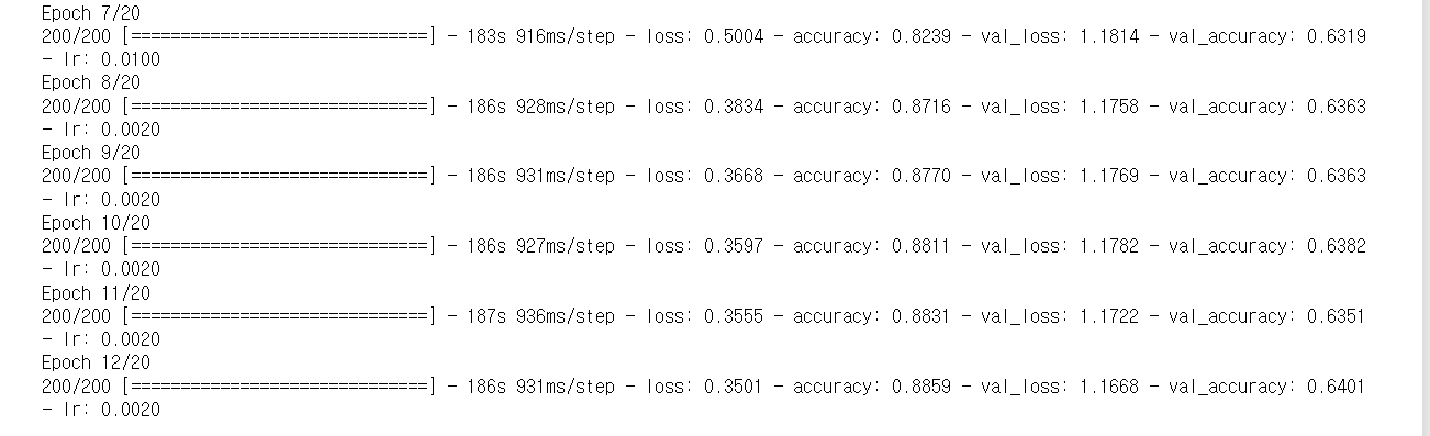
성능 향상을 위해 epoch 수 증가와 학습률 스케줄링을 적용해주었다.

import tensorflow as tf
from tensorflow.keras import layers, models, optimizers
from tensorflow.keras.preprocessing.image import ImageDataGenerator
from tensorflow.keras.callbacks import ReduceLROnPlateau, EarlyStopping
import os

# 데이터 로드
directory = os.path.join(os.getcwd(), 'dataset/')
image_size = (224, 224)
batch_size = 32

datagen = ImageDataGenerator(
    rescale=1./255,
    validation_split=0.2)

train_generator = datagen.flow_from_directory(
    directory,
    target_size=image_size,
    batch_size=batch_size,
    class_mode='categorical',
    subset='training')

validation_generator = datagen.flow_from_directory(
    directory,
    target_size=image_size,
    batch_size=batch_size,
    class_mode='categorical',
    subset='validation')

# 모델 불러오기
base_model = tf.keras.applications.MobileNetV2(input_shape=(224,224,3), include_top=False, weights='imagenet')
base_model.trainable = False

model = tf.keras.Sequential([
  base_model,
  layers.GlobalAveragePooling2D(),
  layers.Dense(8, activation='softmax')  # 클래스 수를 8개로 변경
])

# 손실함수, 최적화함수 설정
model.compile(optimizer=tf.keras.optimizers.SGD(lr=0.001, momentum=0.9),
              loss='categorical_crossentropy',
              metrics=['accuracy'])

# 학습률 조정과  early stop을 위한 콜백 설정
reduce_lr = ReduceLROnPlateau(monitor='val_loss', factor=0.2, patience=5, min_lr=0.001)
early_stopping = EarlyStopping(monitor='val_loss', patience=10)

# 학습
history = model.fit(train_generator, 
                    epochs=20,
                    validation_data=validation_generator,
                    callbacks=[reduce_lr, early_stopping])

# 모델 가중치 저장
model.save_weights('classification.h5')