• Matplotlib's default tick locators and formatters are designed to be generally sufficient in many common situations, but are in no way optimal for every plot.
  
  
• Matplotlib aims to have a Python object representing everything that appears on the plot: for example, recall that the Figure is the bounding box within which plot elements appear.
• Each Matplotlib object can also act as a container of subobjects: for example, each Figure can contain one or more Axes objects, each of which in turn contains other objects representing plot contents.
• The tickmarks are no exception. Each axes has attributes xaxis and yaxis, which in turn have attributes that contain all the properties of the lines, ticks, and labels that make up the axes.

Major and Minor Ticks

• Within each axes, there is the concept of a major tickmark, and a minor tickmark.
• As the names imply, major ticks are usually bigger or more pronounced, while minor ticks are usually smaller.
• By default, Matplotlib rarely makes use of minor ticks, but one place you can see them is within logarithmic plots.

# In[1]
import matplotlib.pyplot as plt
plt.style.use('classic')
import numpy as np

%matplotlib inline

---

# In[2]
ax=plt.axes(xscale='log',yscale='log')
ax.set(xlim=(1,1E3),ylim=(1,1E3))
ax.grid(True);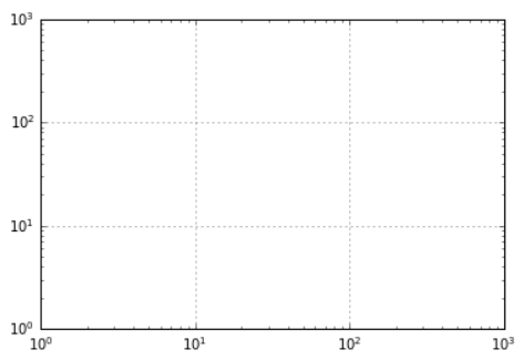

• In this chart each major tick shows a large tickmark, label, and gridline, while each minor tick shows a smaller tickmark with no label or gridline.
  
  
• These tick properties - locations and labels, that is - can be customized by setting the formatter and locator objects of each axis.

# In[3]
print(ax.xaxis.get_major_locator())
print(ax.xaxis.get_minor_locator())
print('\n')
print(ax.xaxis.get_major_formatter())
print(ax.xaxis.get_minor_formatter())

# Out[3]
<matplotlib.ticker.AutoLocator object at 0x7f5ae12edf00>
<matplotlib.ticker.NullLocator object at 0x7f5ae12eeb60>


<matplotlib.ticker.ScalarFormatter object at 0x7f5ae12eebc0>
<matplotlib.ticker.NullFormatter object at 0x7f5ae12ef160>

Hiding Ticks or Labels

• Perhaps the most common tick/label formatting operation is the act of hiding ticks or labels.
• This can be done using plt.NullLocator and plt.NullFormatter.

# In[4]
ax=plt.axes()
rng=np.random.default_rng(1701)
ax.plot(rng.random(50))
ax.grid()

ax.yaxis.set_major_locator(plt.NullLocator())
ax.xaxis.set_major_formatter(plt.NullFormatter())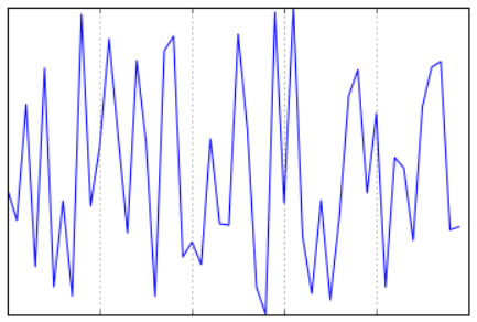

• We've removed the labels (but kept the ticks/gridlines) from the x-axis, and removed the ticks (and thus the labels and gridlines as well) from the y-axis.
• Having no ticks at all can be useful in many situations - for example, when you want to show a grid of images.

# In[5]
fig,ax=plt.subplots(5,5,figsize=(5,5))
fig.subplots_adjust(hspace=0,wspace=0)

# get some face data from Scikit-Learn
from sklearn.datasets import fetch_olivetti_faces
faces=fetch_olivetti_faces().images

for i in range(5):
    for j in range(5):
        ax[i,j].xaxis.set_major_locator(plt.NullLocator())
        ax[i,j].yaxis.set_major_locator(plt.NullLocator())
        ax[i,j].imshow(faces[10 * i + j],cmap='binary_r')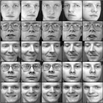

• Even image is shown in its own axes, and we've set the tick locators to null because the tick values do not convey relevant information for this particular visualization.

Reducing or Increasing the Number of Ticks

• One common problem with the default settings is that smaller subplots can end up with crowded labels.

# In[6]
fig,ax=plt.subplots(4,4,sharex=True,sharey=True)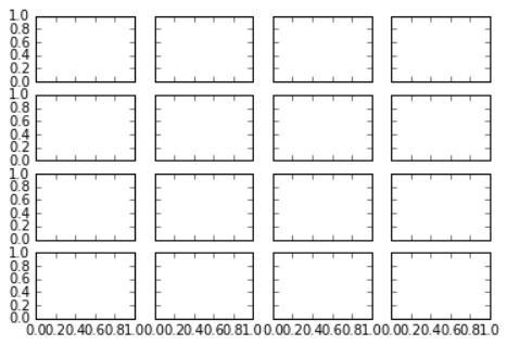

• Particularly for the x-axis ticks, the numbers nearly overlap, making them quite difficult to decipher(판독하다).
• One way to adjust this is with plt.MaxNLocator, which allows us to specify the maximum number of ticks that will be displayed.
• Given this maximum number, Matplotlib will use internal logic to choose the particular tick locations.

# In[7]
# for every axis, set the x and y major locator
for axi in ax.flat:
    axi.xaxis.set_major_locator(plt.MaxNLocator(3))
    axi.yaxis.set_major_locator(plt.MaxNLocator(3))
fig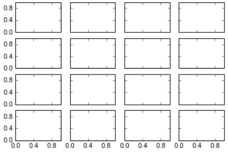

• If you want even more control over the locations of regularly spaced ticks, you might also use plt.MultipleLocator.

Fancy Tick Formats

• Matplotlib's default tick formatting can leave a lot to be desired: it works well as a broad default, but sometimes you'd like to do something different.

# In[8]
# plot a sine and cosine curve
fig,ax=plt.subplots()
x=np.linspace(0,3 * np.pi,1000)
ax.plot(x,np.sin(x),lw=3,label='Sine')
ax.plot(x,np.cos(x),lw=3,label='Cosine')

# set up grid, legend, and limits
ax.grid(True)
ax.legend(frameon=False)
ax.axis('equal')
ax.set_xlim(0,3 * np.pi);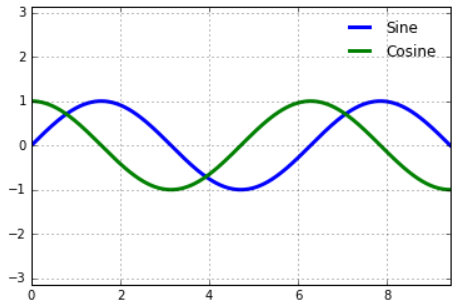

• There are a couple of changes we might like to make here.
• First, it's more natural for this data to space the ticks and gridlines in multiples of $\pi$. We can do this by setting a MultipleLocator, which locates ticks at a multiple of the number we provide.
• For good measue, we'll add both major and minor ticks in multiples of $\pi$/2 and $\pi$/4.

# In[9]
ax.xaxis.set_major_locator(plt.MultipleLocator(np.pi / 2))
ax.xaxis.set_minor_locator(plt.MultipleLocator(np.pi / 4))
fig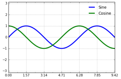

• But now these tick labels look a little bit silly: we can see that they are multiples of $\pi$, but the decimal representation does not immediately convey this.
• To fix this, we can change the tick formatter. There's no built-in formatter for what we want to do, so we'll instead use plt.FuncFormatter, which accepts a user-defined function giving fine-grained control over the tick outputs.

# In[10]
def format_func(value, tick_number):
    # find number of multiple of pi/2
    N=int(np.round(2*value/np.pi))
    if N==0:
        return "0"
    elif N==1:
        return r"$\pi/2$"
    elif N==2:
        return r"$\pi$"
    elif N % 2 > 0:
        return rf"${N}\pi/2$"
    else:
        return rf"${N//2}\pi$"

ax.xaxis.set_major_formatter(plt.FuncFormatter(format_func))
fig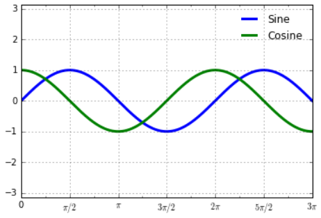

• We've made use of Matplotlib's LaTeX support, specified by enclosing the string within dollar signs.
• This is very convenient for display of mathematical symbols and formulae: you can use this like markdown syntax.

Summary of Formatters and Locators

• We've seen a couple of the available formatters and locators; I'll conclude this chapter by listing all of the built-in locator options and formatter options.

Matplotilb locator options

Locator class	Description
NullLocator	No ticks
FixedLocator	Tick locations are fixed
IndexLocator	Locator for index plots
LinearLocator	Evenly spaced ticks from min to max
LogLocator	Logarithmically spaced ticks from min to max
MultipleLocator	Ticks and range are a multiple of base
MaxNLocator	Finds up to a max number of ticks at nice locations
AutoLocator	(Default) MaxNLocator with simple defaults
AutoMinorLocator	Locator for minor ticks

Matplotlib formatter options

Formatters class	Description
NullFormatter	No labels on the ticks
IndexFormatter	Set the strings from a list of labels
FixedFormatter	Set the strings manually for the labels
FuncFormatter	User-designed function sets the labels
FormatStrFormatter	Use a format string for each value
ScalarFormatter	Default formatter for scalar values
LogFormatter	Default formatter for log axes