
머신러닝을 하기 전에 데이터 전처리가 잘 되어야 한다.
일반적으로 머신러닝을 하려면 데이터 전처리 과정이 80%, 머신러닝 20% 정도라고 생각하면 된다.
강사님께서 머신러닝에서 자주 사용되는 데이터 전처리 과정을 전처리 과정을 강의해 주시고 머신러닝에 대한 설명을 해주셨다.
1. 데이터 전처리
머신러닝에 자주 사용하는 데이터 전처리하는 방법
- (1) 불필요한 변수를 제거
- (2) NaN 삭제
- NaN 포함된 행 제거
- NaN 포함된 변수 제거
- (3) NaN 채우기
- 평균값으로 채우기
- 최빈값으로 채우기
- 앞/뒤 값으로 채우기(시계열의 경우)
- 선형 보간법으로 채우기
- (4) 가변수화
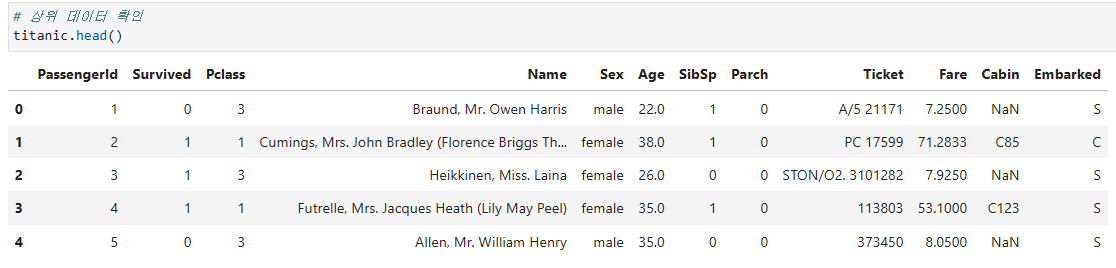
(1) 불필요한 변수 제거 - drop()
타이타닉 데이터 중 Cabin은 결측치가 77.1%정도이고 Passengerid, Name, Ticket은 유니크한 값이므로 제거함
- 기존 데이터 구성
# 여러 열 동시 제거
drop_cols = ['Cabin', 'PassengerId', 'Name', 'Ticket']
titanic.drop(drop_cols, axis=1, inplace=True)
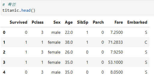
# 확인
titanic.head()- 불필요한 변수 제거 됨
(2) NaN 삭제
# 결측치 확인
titanic.isna().sum() 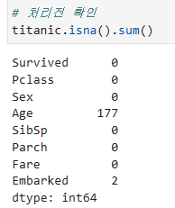
- 결측치
Age,Embarked변수에 각각 177개, 2개 존재 - 머신러닝을 돌리려면 처리가 필요함
1) NaN 포함된 행 제거 - dropna(axis=0)
# NaN이 포함된 모든 행(axis=0) 제거 (행 방향으로 날림)
titanic.dropna(axis=0, inplace=True)

# 확인
titanic.isna().sum() 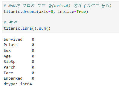
- 결측치가 포함된 행을 제거하여 결측치 처리됨
2) NaN 포함된 변수 제거 - dropna(axis=1)
# NaN 열이 포함된 모든 변수(axis=1) 제거
titanic.dropna(axis=1, inplace=True)

# 확인
titanic.isna().sum()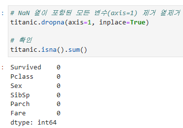
- 결측치가 포함된
Age,Embarked변수 제거 됨
(3) NaN 채우기
1) 평균값으로 채우기 - fillna()
# Age 평균 구하기
mean_age = titanic['Age'].mean()

# NaN을 평균값으로 채우기
titanic['Age'].fillna(mean_age, inplace=True)

# 확인
titanic.isna().sum()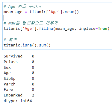
Age변수의 결측치를 평균으로 채움
2) 최빈값으로 채우기
# Embarked 변수 값 확인 value_counts()
titanic['Embarked'].value_counts(dropna=True) # dropna = True는 결측치를 빼고 보여줌 (디폴트값)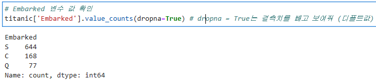
최빈값 확인 - value_counts.idxmax() / mode()
# 최반값 확인 #1
titanic['Embarked'].value_counts(dropna=True).idxmax()
> # 출력
'S'

# 최빈값 확인 #2
titanic['Embarked'].mode()[0]
> # 출력
'S'
최빈값으로 채우기
# NaN 값을 가장 빈도가 높은 값으로 채우기
# titanic['Embarked'].fillna('S', inplace=True)

freq_emb = titanic['Embarked'].mode()[0]
titanic['Embarked'].fillna(freq_emb, inplace=True)

# 확인
titanic.isna().sum()
3) 앞/뒤 값으로 채우기(시계열의 경우)
- 시계열 데이터인 경우 많이 사용하는 방법
- method='ffill': 바로 앞의 값으로 채우기
- method='bfill': 바로 뒤의 값으로 채우기
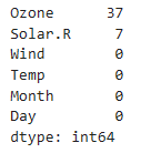
# 결측치 확인
air.isna().sum()Ozone,Solar.R에 결측치 존재
# Ozone 변수 NaN 값을 바로 앞의 값으로 채우기
air['Ozone'].fillna(method='ffill', inplace=True)

# Solar.R 변수 NaN 값을 바로 뒤의 값으로 채우기
air['Solar.R'].fillna(method='bfill', inplace=True)

# 확인
air.isna().sum()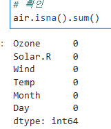
- 결측치가
Ozone,Solar.R은 각각 앞의 값과 뒤의 값으로 채워짐
4) 선형 보간법으로 채우기 - interpolate()
interploate(method='linear')
# 선형 보간법으로 채우기
# air['Ozone'].interpolate(method='linear', inplace=True)
# air['Solar.R'].interpolate(method='linear', inplace=True)

air.interpolate(method='linear', inplace=True)
# 어떤 것이 결측치가 있는 데이터인지 알아서 이렇게 가능

# 확인
air.isna().sum()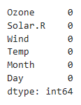
(4) 가변수화 - get_dummies()
get_dummies(data, columns=, drop_first=, dtype= )
# 가변수 대상 변수 식별
dumm_cols = ['Pclass', 'Sex', 'Embarked']


# dtype 안하면 T/F로 나옴
# titanic = pd.get_dummies(titanic, columns=dumm_cols, drop_first=True)

# 가변수화
titanic = pd.get_dummies(titanic, columns=dumm_cols, drop_first=True, dtype=int)

# 확인
titanic.head()
2. 머신러닝 (개념)
(1) 용어 및 개념정리
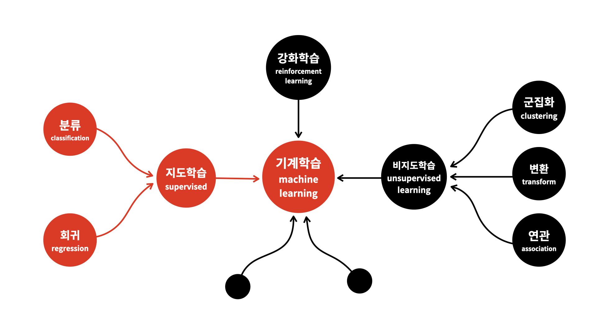
1) 학습 방법에 따른 분류
지도학습 - 학습 대상 데이터에 정답을 주고 데이터의 패턴을 배우게 하는 학습 방법
비지도학습 - 정답이 없는 데이터 만으로 배우게 하는 학습 방법
강화학습 - 선택한 결과에 대해 보상을 받아 행동을 개선하면서 배우게 하는 학습 방법
2) 과제에 따른 분류
분류 문제(Classification) - 분류 규칙을 찾고 그 규칙을 기반으로 새롭게 주어진 데이터를 분류하는 것(지도학습)
회귀 문제(Regression) - 입력값과 결과값의 연관성을 찾고, 그 연관성을 기반으로 새롭게 주어진 데이터에 대한 값을 예측하는 것(지도학습)
클러스터링(Clustring) - 주어진 데이터를 학습하여 분류 규칙을 찾아 데이터를 분류함, 정답이 없어 성능평가가 어려움 (비지도학습)
3) 머신러닝 분류
- 오늘은 분류방식과 회귀방식을 진행한다.
(2) 분류와 회귀 구분
- 분류(Classification)는 범주값을 예측하는 것이다.
- 회귀(Regression)는 연속적인 숫자를 예측하는 것이다.
- 두 값 사이에 중간값이 의미가 있는 숫자인지
- 두 값에 대한 연산 결과가 의미가 있는 숫자인지
예시
1. 고객의 타 통신사로 이동할까? - 분류
2. 내일 주가가 오를까? - 회귀
3. 내일 주가가 얼마일까? - 분류
1) 분류
분류 알고리즘
- DecisionTreeClassifier
- KNeighborsClassifier
- LogisticRegression
- RandomForestClassifier
- XGBClassifier
분류 모델 평가
- accuracy_score
- recall_score
- precision_score
- classification_report
- confusion_matrix
2) 회귀
회귀 알고리즘
- LinearRegression
- KNeighborsRegressor
- DecisionTreeRegressor
- RandomForestRegressor
- XGBRegressor
회귀 모델 평가
- mean_absolute_error
- mean_squared_error
- root mean_squared_error
- mean_absolute_percentage_error
- r2_score
- 코드 작성할때 팁을 주자면 직접 입력하다 오타내지말고 tab을 이용하는 걸 추천한다!
- 대신 어떤 상황에 어떤 방법을 쓸지 생각하고 쓰자
3. 머신러닝 (실습)
(1) 데이터 분리 및 모델링 구조
- 데이터프레임을 x와 y를 분리
target = '타겟변수'
x = data.drop(target, axis=1)
y = data.loc[:, target]- 학습용과 평가용 데이터를 분리
from sklearn.model_selection import train_test_split
x_train, x_test, y_train, y_test = train_test_split(x, y, test_size= 0.3)- 불러오기
from sklearn.linear_model import LinearRegression
from sklearn.metrics import mean_absolute_error- 선언하기
model = LinearRegression()- 학습하기
model.fit(x_train, y_train)- 예측하기
y_pred = model.predict(x_test)- 평가하기
mean_absolute_error(y_test, y_pred)(2) 예제 실습
- 오존 농도를 예측할 수 있는 머신러닝 모델을 만들거다.
- 오존 농도를 예측하는 것은 회귀분석이다
1) 데이터 이해
data.head()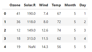
- 이 데이터는 시계열 데이터이고, 5개의 독립변수와 1개의 종속변수(
Ozone)가 있다.
- head, tail, info, describe, corr 과 같은 함수를 사용하여 데이터에 대한 이해가 필요하다.
- 아래와 같이 상관관계를 시각화하여
Ozone변수와 어떤게 관계가 있는지 알 수 있다.
# 상관관계 시각화
sns.heatmap(data.corr(numeric_only = True),
            annot = True, # 숫자 생성
            cmap='Blues', # 색 정함
            cbar=False, # 우측 컬러바 안보이게 함
            square = True, # 정사각형 출력
            fmt='.2f', # 소수점 자리수 2째자리 까지
            annot_kws={'size': 9} # 사이즈 정해줌
           )
plt.show()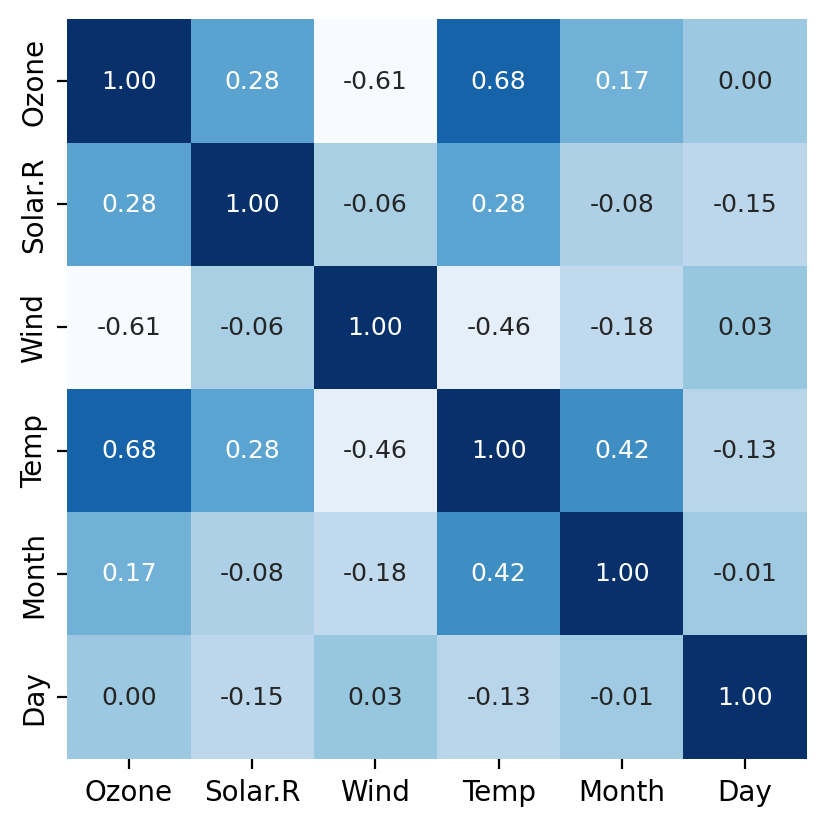
2) 결측치 처리
# 결측치 확인
data.isna().sum()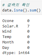
- Solar.R에 결측치가 있는 것을 확인
# 전날 값으로 결측치 채우기
data.fillna(method='ffill', inplace=True)method='ffill'로 전날 값으로 결측치를 채웠음
3) 변수 제거
- 분석에 의미가 없다고 판단되는 변수를 제거함
# 변수 제거
drop_cols = ['Month', 'Day'] # 삭제할 열 선택
data.drop(drop_cols, axis=1, inplace=True) # axis=1 열 삭제
4) x, y 분리
# target 확인
target = 'Ozone'

# 데이터 분리
x = data.drop(target, axis=1) # 타겟 열을 제외한 데이터를 x에 저장
y = data.loc[:, target] # 모든 행, target 열 만
5) 학습용, 평가용 데이터 분리
# 모듈 불러오기
from sklearn.model_selection import train_test_split

# 7:3으로 분리
x_train, x_test, y_train, y_test = train_test_split(x, y,
													test_size=0.3,
                                                    random_state=1)
                                              # shuffle=False 시계열 데이터의 경우 섞으면 안될때 사용
                                             # stratify=y 균일하게 배분함 => 불균형데이터에서 많이 사용함
test_size=0.3 는 70% 30%로 분류함
test_size=3 이면 마지막 3개를 의미함
6) 모델링
알고리즘: LinearRegression
평가방법: mean_absolute_error
이 방법으로 함
# 1단계 불러오기
from sklearn.linear_model import LinearRegression
from sklearn.metrics import mean_absolute_error

# 2단계 선언하기
model = LinearRegression()

# 3단계 학습하기
model.fit(x_train, y_train)

# 4단계 예측하기
y_pred = model.predict(x_test)

# 5단계 평가하기
print(f'MAE: {mean_absolute_error(x_test, y_pred)}')
>
MAE: 13.976843190385708


# 시각화
plt.plot(y_test.values, label='Actual')
plt.plot(y_pred, label='Predicted')
plt.legend()

plt.show()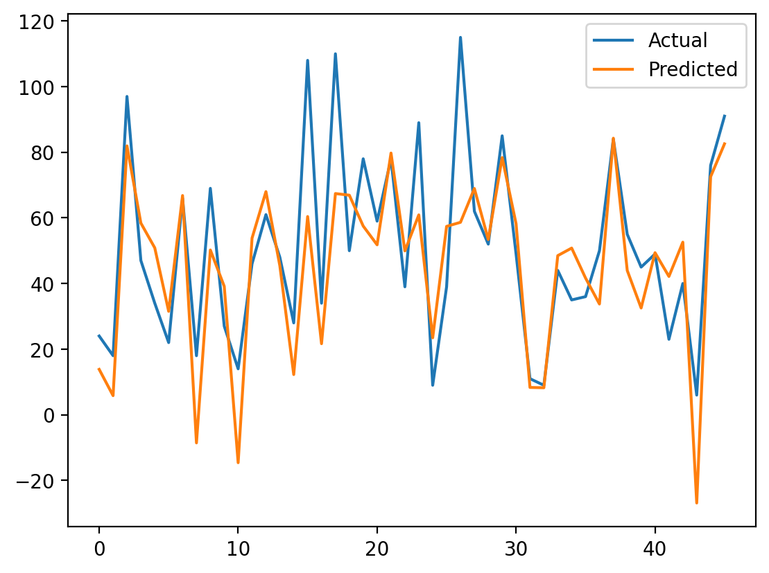
회고
오늘은 파이썬에서 머신러닝으로 처음 모델을 만들어봤다.
생각보다 재밌고 같은 방법을 반복하는 느낌이다. 오늘 하면서 느낀건 머신러닝 코딩방법은 어렵진 않은 것 같다.
반복만하면 되고 어떤 알고리즘을 사용할지와 결과물에 대한 나의 분석능력을 길러야겠다는 생각이 든다.
내일은 예비군 이슈로 늦을 예정..ㅇㅅㅇ