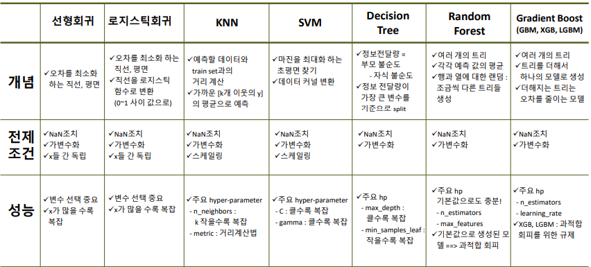
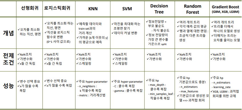
1.머신러닝 복습
평가지표
회귀모델 :
MSE, RMSE, MAE , MAPE(오차율) , R2 score
- 비즈니스에서 사용할 수 있는 평가 지표 : MAE , MAPE
- MAE : 예측값과 실제값의 차이에 대한 평균, 오차를 측정하는 방법은 단위에 따라 달라지므로 비즈니스적으로 해석해야함
- 1-MAPE = 1- 오차율 = 정확율
분류모델 :
confusion matrix ( accuracy , recall , precision , f1-score)
중요도는?
recall> precision
: 거짓음성을 최소화하고 실제 양성 샘플을 놓치지 않기 위해
: 비즈니스적으로 차이가 있기 때문에 해석 방식 및 도메인 지식에 따라 평가 방식 다름
2.딥러닝 개념 이해
머신러닝과 딥러닝의 차이점
전처리 : 스케일링 필수
모델링 : 모델 구조 생성 -> 컴파일 -> 학습 -> 학습 곡선 확인 -> 예측 및 성능 평가
딥러닝 코드
1) 데이터 전처리
- 가변수화 & 데이터스케일링
2) 모델링 - 모델 설계 & 컴파일 & 모델 학습 및 검증
: 가중치에 초기값을 할당한 이후, 오차를 계산하고 줄이는 방향으로 가중치를 조정해야한다. 오차의 변동이 없으면 끝내면 되지만, 1번째 단계로 돌아가 오차를 최소화하도록 반복한다.
이때 가중치의 폭을 줄이는 파라미터는 ? learning rate
반복횟수는? epochs
오차를 계산? loss
from keras.models import Sequential
from keras.layers import Dense
from keras.backend import clear_session

path = 'https://raw.githubusercontent.com/DA4BAM/dataset/master/advertising.csv'
adv = pd.read_csv(path)
adv.head()

target = 'Sales'
x = adv.drop(target, axis=1)
y = adv.loc[:, target]

x_train, x_val, y_train, y_val = train_test_split(x, y, test_size=.2, random_state = 20)

scaler = MinMaxScaler()
x_train = scaler.fit_transform(x_train)
x_val = scaler.transform(x_val)
# min max sclaer : 최소 0으로 / 최대 1로 맞춰줌

nfeatures = x_train.shape[1] #num of columns
nfeatures #열개수

# 메모리 정리
clear_session()

# Sequential 타입 모델 선언
model = Sequential( Dense(1, input_shape = (nfeatures,))  )
#input_shape : 예측 단위 데이터

# 모델요약
model.summary()

# 컴파일 : 컴퓨터가 이해하는 언어로 변환
model.compile(optimizer='adam', loss='mse')

model.fit(x_train,y_train)

pred =model.predict(x_val)

print(f'RMSE  : {mean_squared_error(y_val, pred, squared=False)}')
print(f'MAE   : {mean_absolute_error(y_val, pred)}')
print(f'MAPE  : {mean_absolute_percentage_error(y_val, pred)}')
학습 절차 시각화 코드
def dl_visualize(ep, lr) :
    clear_session()

    model = Sequential([ Dense(1, input_shape = (1,)) ])

    model.compile(loss='mse', optimizer= Adam(learning_rate = lr))
    mcp = ModelCheckpoint(filepath='/content/{epoch:d}.h5',
                        monitor='val_loss', save_best_only=False, save_weights_only=True)

    history = model.fit(x_train_s, y_train_s, verbose = 0, epochs = ep, callbacks=[mcp]).history

    coef,intercept = [],[]

    for i in range(ep) :
        file = f'/content/{i+1}.h5'
        model.load_weights(file)
        coef.append(np.array(model.weights[0])[0,0])
        intercept.append(np.array(model.weights[1])[0])

    plt.figure(figsize = (20,8))
    plt.subplot(1,2,1)
    sns.scatterplot(x=x_train_s.reshape(-1,), y=y_train_s, alpha = .5)
    plt.grid()
    plt.xlabel('lstat')
    for i in range(ep):
        x = np.linspace(0,1,10)
        y = coef[i]*x+ intercept[i]
        plt.plot(x, y, 'r--')
        v = 1.005
        plt.text(v, coef[i]*v+ intercept[i], f'ep:{i+1}', color = 'r')

    plt.subplot(1,2,2)
    plt.plot(range(1, ep+1), history['loss'], label='train_err', marker = '.')

    plt.ylabel('Loss')
    plt.xlabel('Epoch')
    plt.legend()
    plt.grid()
    plt.show()
학습곡선 그래프 함수
# 함수로 만들어서 사용합시다.
def dl_history_plot(history):
    plt.figure(figsize=(10,6))
    plt.plot(history['loss'], label='train_err', marker = '.')
    plt.plot(history['val_loss'], label='val_err', marker = '.')

    plt.ylabel('Loss')
    plt.xlabel('Epoch')
    plt.legend()
    plt.grid()
    plt.show()
3.딥러닝 모델링 : regression
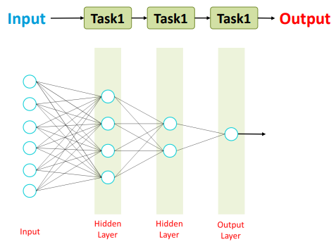
딥러닝 구조 : hidden layer
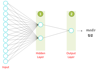
- input과 output 사이에 있는 것은 모두 hidden layer
- 모델 설계과정에서 hidden layer 설정
- hidden layer가 없다면 선형회귀에 불과하다
: 이때 활성함수를 '비선형 함수'로 사용하는 이유는?
: 은닉층 네트워크가 똑같은 기능을 하지 않기 위해 신경망 층을 깊게 하기 위해서는 시그모이드,relu함수를 활용해야한다.
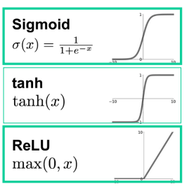
대표적인 비선형함수는 다음과 같다.
-
hidden layer을 사용하는 이유는?
: 선형 함수를 비선형함수로 변환해주기 위해서 -
input shape은 1번째 layer 에서 사용
: 히든 레이어는 활성함수를 필요로 함 (relu함수 일반적)
# 메모리 정리
clear_session()

# Sequential 타입 모델 선언(입력은 리스트로!)
model3 = Sequential([  Dense(2, input_shape = (nfeatures,), activation = 'relu'),
                       Dense(1)   ])

# 모델요약
model3.summary()
compile
컴파일이란? 컴퓨터가 이해할 수 있는 형태로 변환하는 작업
1) 오차함수:
오차계산을 무엇으로 할지 결정
2) optimizer:
오차를 최소화하도록 가중치를 조절하는 역할
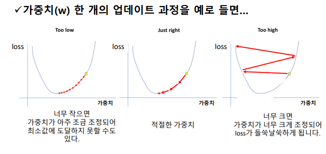
learning rate 설정 중요
너무 작을 경우, 가중치가 조금 조정되어 지역 최적해 발생 -> 최솟값에 미치지 못할 수 있음
너무 클 경우, 가중치가 너무 크게 조정되어 loss 값 영향
학습
반복횟수(epochs)와 validation split을 통해 모델 학습
learning rate값이 너무 작을 경우 ,epochs 값을 늘려 조정
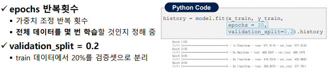
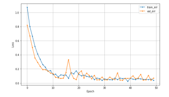
이후 학습곡선을 통해 valerr와 train err 값 확인
그래프를 통해 과적합 되었는지 확인 가능하며 최적의 epochs 선정 가능
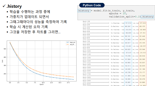
바람직한 곡선 모습은?
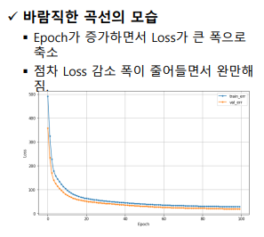
epoch이 증가하면서 loss가 축소하는 모습
과적합된 곡선의 모습은?
: learning rate와 epochs 둘 다 조정 필요
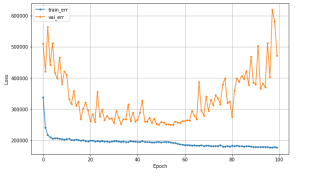
적합은 잘 되었지만 오차 폭을 줄여야하는 경우는?
: 가중치 폭을 조정하는 leanring rate 값을 줄여 해결 가능