코딩 돌려보기(2일차 실습답안 & 회귀 따릉이)
회귀: 하이퍼 파라미터
#라이브러리 설치
!pip install keras-tuner

# 라이브러리 로딩
import matplotlib.pyplot as plt
import numpy as np
import pandas as pd
import seaborn as sns

# Make NumPy printouts easier to read.
np.set_printoptions(precision=3, suppress=True)

from keras.layers import Dense, Conv2D, MaxPool2D, Conv1D, MaxPool1D, Normalization, Reshape,Flatten
from keras.models import Sequential
from keras.backend import clear_session
from keras.optimizers import Adam
from sklearn.metrics import *
from sklearn.preprocessing import MinMaxScaler
import kerastuner as kt
- 딥러닝에서도 하이퍼 파라미터가 가능하다.
- kerastuner 라이브러리를 활용함으로써 하이퍼 파라미터 튜닝을 진행할 수 있다.
# 학습곡선 함수
def dl_history_plot(history):
    plt.plot(hist['loss'], marker = '.', label = 'train_acc')
    plt.plot(hist['val_loss'], marker = '.', label = 'val_acc')
    plt.ylabel('loss')
    plt.xlabel('Epoch')
    plt.legend()
    plt.grid()
    plt.show()

url = 'http://archive.ics.uci.edu/ml/machine-learning-databases/auto-mpg/auto-mpg.data'
column_names = ['MPG', 'Cylinders', 'Displacement', 'Horsepower', 'Weight',
                'Acceleration', 'Model Year', 'Origin']

raw_dataset = pd.read_csv(url, names=column_names,
                          na_values='?', comment='\t',
                          sep=' ', skipinitialspace=True)

data = raw_dataset.copy()
data.tail()

#결측치 처리
data.isna().sum()
data = data.dropna()
#가변수화
data['Origin'] = data['Origin'].map({1: 'USA', 2: 'Europe', 3: 'Japan'})
data = pd.get_dummies(data, columns=['Origin'], prefix='', prefix_sep='')
data.tail()
#데이터분할
train = data.sample(frac=0.8, random_state=0)
test = data.drop(train.index)
x_train = train.copy()
x_test = test.copy()

y_train = x_train.pop('MPG')
y_test = x_test.pop('MPG')

#스케일링
scaler = MinMaxScaler()
x_train = scaler.fit_transform(x_train)
x_test = scaler.transform(x_test)
하이퍼 파라미터로 hidden layer의 한 층에서 여러개의 노드를 생성하여 최적의 신경망 층과 MSE 값을 확인해볼 수 있다.
첫번째 케이스는 hidden layer 2개를 튜닝하는 작업이다.
튜닝 방식 : GridSearch
실험 : 총 15회
노드1 : 16, 32, 64, 128, 256
노드2 : 8, 16, 32, 64,128
학습률 : 0.0001, 0.001, 0.01
#튜닝 함수 생성
#수정후
def build_model(hp):
    n1 = hp.Choice('node1', [16, 32, 64, 128, 256])
    n2 = hp.Choice('node1', [8, 16, 32, 64,128])
    model = Sequential([ Dense(units=n1,
                               input_shape = (x_train.shape[1],), activation='relu'),
                         Dense(units=n2,
                               activation='relu'),
                         Dense(1)])
    model.compile(loss='mean_absolute_error', optimizer=Adam(learning_rate = 0.001))
    return model


#튜닝 : random search
%%time

# 랜덤 서치 튜닝 작업 진행
%%time
tuner = kt.RandomSearch(build_model, objective='val_loss', max_trials = 2, project_name='dnn_tune_3')
tuner.search(x_train, y_train, epochs = 30, validation_split = .2, verbose=0)
best_model = tuner.get_best_models(num_models=1)[0]

#summary
tuner.results_summary()

# 튜닝 모델을 이용하여 예측하고 평가하기
pred2_2 = best_model.predict(x_test, verbose = 0)
print('MAE :', mean_absolute_error(y_test, pred2_2))

plt.scatter(y_test, pred2_2)
plt.plot(y_test, y_test, color = 'gray', linewidth = .5)
plt.grid()
plt.show()
튜닝 방식 : GridSearch
실험 : 총 20회
노드1 : 16, 32, 64, 128, 256
노드2 : 8, 16, 32, 64,128
노드3 : 4, 8, 16, 32, 64
학습률 : 0.0001, 0.001, 0.01
- hp.Choice에 각 노드를 할당
- best_model: 최적의 모델 확인 (tuner.get_best_models)
def build_model(hp):
    model = Sequential([ Dense(units=hp.Choice('node1', [16, 32, 64, 128, 256]), input_shape = (x_train.shape[1],), activation='relu'),
                         Dense(units=hp.Choice('node2', [8, 12, 32, 64, 128]), activation='relu'),
                         Dense(units=hp.Choice('node3', [4, 8, 12, 32, 64]), activation='relu'),
                         Dense(1)])
    model.compile(loss='mean_absolute_error', optimizer=Adam(learning_rate = hp.Choice('learning_rate', [0.0001, 0.001, 0.01])))
    return model코드를 입력하세요

# random search

%%time
tuner = kt.RandomSearch(build_model, objective='val_loss', max_trials = 20, project_name='dnn_tune_4')
tuner.search(x_train, y_train, epochs = 100, validation_split = .2, verbose=0)

#최적의 best model 확인
best_model = tuner.get_best_models(num_models=1)[0]

#노드 확인(모든 요소)
tuner.results_summary()

#최적의 모델 확인
#MAE값을 통해서
pred2_3 = best_model.predict(x_test, verbose = 0)
print('MAE :', mean_absolute_error(y_test, pred2_3))

plt.scatter(y_test, pred2_3)
plt.plot(y_test, y_test, color = 'gray', linewidth = .5)
plt.grid()
plt.show()
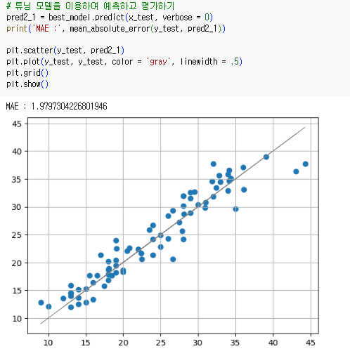
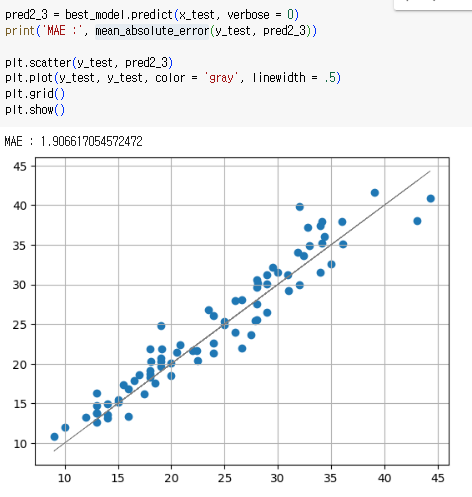
튜닝작업을 더 깊게 했을 때
MAE : 1.9797304226801946
MAE : 1.906617054572472
으로 감소함을 확인
1. feature representation
- hidden layer에서는..?
: 모든 노드간에 연결을 제어할 수 도 있으며, 연결을 제어할 수도 있다.
: 이때 우리는 오차를 줄이는게 목적이며 가중치(파라미터)를 중간 중간 업데이트함으로써 예측값과 실제값과의 격차를 줄여나가야한다.
: loss function으로 오차를 계산한다.
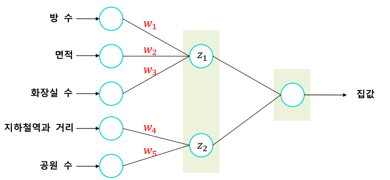
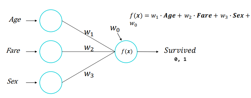
여기서 w1 ~ w3은 내부요인, w4 ~ w5은 외부요인이라고 본다.
내부요인 점수와 외부요인 점수의 가중치를 다르게 두어야하며, 최종 집값을 예측하는데 내부를 0.7 , 외부를 0.3으로 놓는다고 가정해보자.
이때 딥러닝은 머신러닝과 다르게 자동적으로 오차를 최소화하도록 학습을 하며, feature enginnering이 진행되었다.
deeplearning 을 representation learning 이라고 부르는 이유이다.
2.분류 - 이진 분류
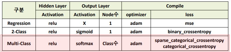
노드의 결과를 활성함수로 변환해야한다.
(why? 확률로 출력해야하며,은닉층의 결과를 풍성하게 만들기 위해서는 단층을 생성할 수 있는 비선형함수가 필요하다= 깊이 있는 학습을 위해서는 hidden layer을 여러 층을 쌓을 수 있는 역할이 필요하다.)
-> hidden layer: relu함수
-> output layer: 이진분류는 sigmoid/다중분류는 softmax
(회귀: x)
이진분류에서의 손실함수 (loss function)
: binary crossentropy

: 이때 이진 분류의 노드 수는 '1'임을 확인하자
3. 분류 - 다중 분류
노드의 수는 y의 범주 수와 같다.
예를 들어, y가 상위/중위/하위로 총 3개의 그룹으로 나뉘어진다면?
y의 개수=3개=노드 수
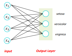
다음과 같은 예시해서도 output layer의 노드 수는 3이다.
마지막 output layer에서 activation을 softmax로 쓴다.
(범주형이므로 비선형함수로 변환하기 위해서)
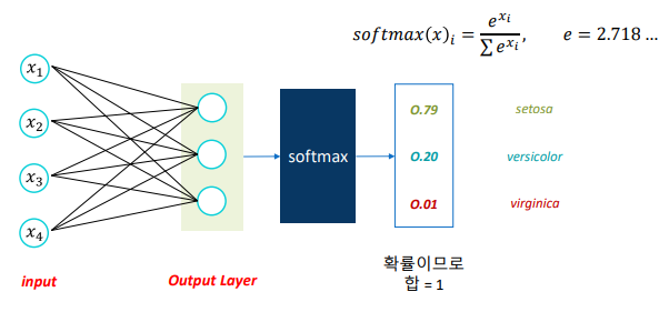
방법
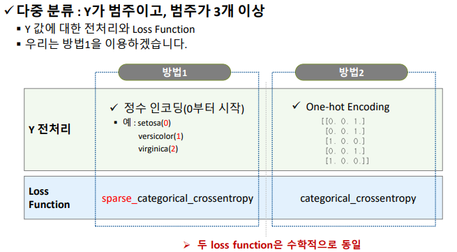
1) Integer Encoding
: 정수 인코딩(라벨 인코딩) + sparse_categorical_crossentropy
: 0부터 시작해서 순차 증가하는 정수로 인코딩
: 자동으로 원핫인코딩하여 처리
2) 원핫 인코딩 + categorical_crossentropy
: 각 클래스에 대한 확률을 출력
: 2차원 구조로 입력을 해야함