Paper Review, ResUNet++ Architecture 이해
ResUNet++ : An Advanced Architecture for Medical Image Segmentation
Paper Summary
-
Task?
Fully automated model for pixel-wise polyp segmentation
이 논문은 픽셀단위로 용종을 segment하는 자동화 모델에 대해서 다루고 있다. -
ResUNet++ Architecture?
Semantic segmentation nueral network that takes advantage of residual blocks, seqeeze and excitation blocks, atrous spatial pyramidal pooling and attention blocks -
Results?
Kvasir-SEG : Dice - 81.33%, mloU - 79.27%
CVC-612 : Dice - 79.55%, mloU - 79.62% 달성
etc
-
Proceedings of the IEEE International Symposium on Multimedia (ISM) 2019에서 발표된 paper 이다.
-
노르웨이 출신 저자는 총 7명으로 5명의 공학자와 2명의 의사로 구성되어 있다. Debesh Jha, Michael A. Riegler, Dag Johansen, P˚al Halvorsen, H˚avard D. Johansen
/ Pia H.Smedsrud, Thomas de Lange -
KVasir-Seg dataset은 기존 KVasir dataset을 소화기내과 전문의인 Pia와 Thomas가 직접 polyp을 annotation하여 생성한 dataset이다. 현재까지도 KVasir, CVC의 조합으로 의료 segmentation 대표적인 benchmark dataset으로 취급하고 있다.
-
논문 발표 당시에는 tensorflow, keras로 코드를 배포한 것을 확인할 수 있고 약 3년 전에 PyTorch로 update한 official code를 upload했다.
ResUNet++ Architecture
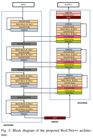
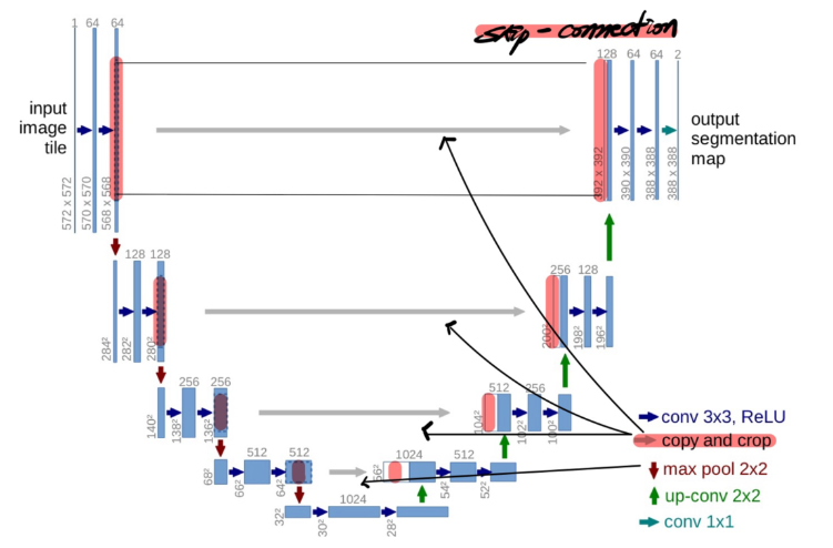
- 전체적인 구조는 Encoding Bridge Decoding으로 세 부분으로 나눌 수 있지만,Bride의 ASPP가 Decoding의 첫번째와 마지막 블록에 도입에 붙어 있다고 볼 수 있기 때문에 간단하게 Encoding, Decoding 두 부분으로 나눠서 이해해볼 수 있다.
Figure에는 나타나 있지 않지만,
class ResUnetPlusPlus:
    def __init__(self, input_size=256):
        self.input_size = input_size

    def build_model(self):
        n_filters = [16, 32, 64, 128, 256]
        inputs = Input((self.input_size, self.input_size, 3))

        c0 = inputs
        c1 = stem_block(c0, n_filters[0], strides=1)

        ## Encoder
        c2 = resnet_block(c1, n_filters[1], strides=2)
        c3 = resnet_block(c2, n_filters[2], strides=2)
        c4 = resnet_block(c3, n_filters[3], strides=2)

        ## Bridge
        b1 = aspp_block(c4, n_filters[4])

        ## Decoder
        d1 = attetion_block(c3, b1)
        d1 = UpSampling2D((2, 2))(d1)
        d1 = Concatenate()([d1, c3])
        d1 = resnet_block(d1, n_filters[3])

        d2 = attetion_block(c2, d1)
        d2 = UpSampling2D((2, 2))(d2)
        d2 = Concatenate()([d2, c2])
        d2 = resnet_block(d2, n_filters[2])

        d3 = attetion_block(c1, d2)
        d3 = UpSampling2D((2, 2))(d3)
        d3 = Concatenate()([d3, c1])
        d3 = resnet_block(d3, n_filters[1])
- code에서 확인할 수 있듯이, Encoder에서는 stride가 2짜리인 ConV layer롤 통해 downsampling을, Decoder에서는 2 times Upsampling을 통해 해상도를 복원했음을 알 수 있다.
Residual Units
-
Why Residual Units?
To improve accuracy, Need deeper neural networks
-> use ResUNet for Backbone Architecture
성능을 높이기 위해서 더 깊은 네트워크를 쌓아야 했고 그렇게 하기 위해서 ResUNet 아키텍처를 백본으로 사용했다. -
Pre-Activation Residual Unit?
기본적으로 ResUNet 에서는 Pre-Activation Residual Unit을 사용했다.
Original : x -> ConV -> BN -> ReLU -> ConV -> BN -> (+x) -> ReLU
ResUNet : x -> BN -> ReLU -> ConV -> BN -> ReLU -> ConV -> (+x)
뒤에 활성화함수가 붙는 Post-Activation 방식보다 더 나은 기울기 흐름을 통해 안정적으로 학습이 가능하게하고 실험적으로 더 좋은 성능을 보이는 경우가 많았다고 한다.
Squeeze & Excitation Units
-
What is Squeeze & Excitation Units?
이 개념이 처음 나온 것은 2017년 마지막 ImageNet Competition에서, 2.53%의 압도적인 성능으로 winning한 Squeeze and Excitation Network의 핵심 구조이다. -
What for?
To ensure network can increase its sensitivity to the relevant features and suppress the unneccessary features.
다시 말해, 좋은 건 살리고 별로 좋지 않은 것은 버리기 위해서.
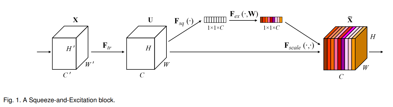
- How it works?
Squeeze는 말 그대로 쥐어 짜내는 것, Excitation은 사전에 쳐보면 활성화, 자극 이런 단어를 뜻하고 있다. 매우 직관적인 명명이라고 생각이 든다. 위에 첨부한 Fig.1에서 확인할 수 있듯이, X가 input으로 들어가면 Feature를 뽑은 U를 얻을 수 있고 여기에 Global Average Pooling을 통해서 11C 짜리를 얻어 낼 수 있다. 이후, 두번의 MLP(multi layer perceptron)을 거친 뒤에 sigmoid를 취해서 Channel 중요도를 얻을 수 있다. 이렇게 얻어낸 중요도를 U에 곱한다.
SE Network를 계승한 Transformer의 attention mechanism?
SE block 구조
Input -> 요약vSqueeze(by GAP) ->MLP&Sigmoid -> 중요도(점수 계산 s) -> 채널별 곱셈
Transformer Attention 구조
Input -> 요약(by Query, Key 내적) -> softmax -> token 점수 계산 -> weighted sum
전체 context를 요약해서 중요도를 계산하고 계산한 점수를 바탕으로 feature를 조절한다는 점에서 Transformer의 Attention mechanism이 SE Network에서의 철학을 공유한다고 볼 수 있지 않을까? 생각해보았다.
정리해보면, Squeeze and Excitation은 마지막에 GAP(Global Average Pooling)로 Squeeze한 채널별 중요도를 가지고 기존 Feature에 곱해주었다는 점에서 channel wise한 attention 이라고도 볼 수 있을 것 같다.
class ResNet_Block(nn.Module):
    def __init__(self, in_c, out_c, stride):
        super().__init__()

        self.c1 = nn.Sequential(
            nn.BatchNorm2d(in_c),
            nn.ReLU(),
            nn.Conv2d(in_c, out_c, kernel_size=3, padding=1, stride=stride),
            nn.BatchNorm2d(out_c),
            nn.ReLU(),
            nn.Conv2d(out_c, out_c, kernel_size=3, padding=1)
        )

        self.c2 = nn.Sequential(
            nn.Conv2d(in_c, out_c, kernel_size=1, stride=stride, padding=0),
            nn.BatchNorm2d(out_c),
        )

self.attn = Squeeze_Excitation(out_c)- 실제로도, 가장 최근에 update한 repo에서 코드를 보면, Squeeze_Excitation(out_c)을 적용하는 함수를 self.attn으로 정의한 부분을 확인할 수 있다.
ASPP, Atrous Spation Pyramidal Pooling
- Why ASPP?
Cause of variational, unruled polypsize, contextual information is caputred at various scales So, need many parrarel atrous convolutions with different rates.
아래에 첨부한 Fig에서 볼 수 있듯이, polyp은 size가 매우 다양하기 때문에, 다양한 스케일에서 캡쳐한 contextual information이 필요하다. 그렇기 때문에 atrous convolution을 다양한 rate에서 적용하여 얻는다.
-
How ASPP works?
variational dilation rate으로 convolution을 여러번 수행해서 다양한 receptive field를 concatenation한다. -
Dilation Convolution?
fixed convolution kernel은 항상 고정된 범위만을 탐색하기 때문에 근처 정보밖에 볼 수 없을 것이다, 하지만 dilation convolution 팽창 합성곱을 사용하게 되면 같은 kernel size라도 또 같은 연산량임에도 불구하고 더 넓은 범위를 보는 효과를 얻을 수 있다.(Receptive Field가 넓어진다.) 또한, pooling처럼 downsample 하지 않기 때문에 해상도의 손실이 없다고 볼 수 있다.
X X X
X X X
X X X  (3*3 kernel)
              ┐
              │
              ▼
X - X - X
- - - - - -
X - X - X
- - - - - -
X - X - X   (3*3 kernel with dilation = 2)
def aspp_block(x, num_filters, rate_scale=1):
x1 = Conv2D(num_filters, (3, 3), dilation_rate=(6 * rate_scale, 6 * rate_scale), padding="same")(x)
x1 = BatchNormalization()(x1)
x2 = Conv2D(num_filters, (3, 3), dilation_rate=(12 * rate_scale, 12 * rate_scale), padding="same")(x)
x2 = BatchNormalization()(x2)
x3 = Conv2D(num_filters, (3, 3), dilation_rate=(18 * rate_scale, 18 * rate_scale), padding="same")(x)
x3 = BatchNormalization()(x3)
x4 = Conv2D(num_filters, (3, 3), padding="same")(x)
x4 = BatchNormalization()(x4)
y = Add()([x1, x2, x3, x4])
y = Conv2D(num_filters, (1, 1), padding="same")(y)
return y- official code에서는 1, 6, 12, 18 네 개의 dilation rate을 사용한 conv를 거쳐 x1, x2, x3, x4를 만들고 forward에 냅다 add해서 concat하는 것을 확인해볼 수 있다.
Attention Units
-
Why Attention Units?
기존 UNet의 문제는 필요없는 정보까지 모두 통째로 전달해버린다는 점이다. 그렇다면 Decoder에게 polyp에 관한 정보만을 전달할 수 없을까? 그래서 나온 것이 "attention unit"이다. skip connection을 filtering해서 중요한 부분만을 주목해서 통과시키는 부분. -
transformer attention에서 영감을 받은 "attention units"
저자는 attention units을 설명하는 마지막 부분에서, " Inspired by the success of attention mechanism, both in NLP and computer vision tasks,
we implemented the attention block in the decoder part of our
architecture to be able to focus on the essential areas of the
feature maps."이라는 샤라웃과 함께 영감을 얻은 출처를 밝히고 있다.
Encoder Feature Map ----┐
                        │ (skip)
                        ▼
                  [Attention Unit] ---> filtered feature → decoder

Decoder Feature Map ----┘  (gating signal)

def attetion_block(g, x):
    """
        g: Output of Parallel Encoder block
        x: Output of Previous Decoder block
    """

    filters = x.shape[-1]

    g_conv = BatchNormalization()(g)
    g_conv = Activation("relu")(g_conv)
    g_conv = Conv2D(filters, (3, 3), padding="same")(g_conv)

    g_pool = MaxPooling2D(pool_size=(2, 2), strides=(2, 2))(g_conv)

    x_conv = BatchNormalization()(x)
    x_conv = Activation("relu")(x_conv)
    x_conv = Conv2D(filters, (3, 3), padding="same")(x_conv)

    gc_sum = Add()([g_pool, x_conv])

    gc_conv = BatchNormalization()(gc_sum)
    gc_conv = Activation("relu")(gc_conv)
    gc_conv = Conv2D(filters, (3, 3), padding="same")(gc_conv)

    gc_mul = Multiply()([gc_conv, x])
return gc_mul- 위 코드에서 확인할 수 있듯이 먼저 Decoder로 부터 g를 전달받고 maxpooling으로 크기를 조절한다. 그 다음 Encoder로 ㅂ터 전달받은 x도 동일하게 ConV로 조절을 시켜준다. 그리고 "Add()[g_pool, x_conv]" 두 input을 componet wise로 섞어서 겹치는 부분을 중요한 부분의 후보로 둔다. 이후 이렇게 합쳐진 feature를 한번 더 ConV를 진행한다. 이렇게 나온 결과를 attention weight으로 주어서 일종의 mask?처럼 원본 skip feature x에 곱해서 attention을 적용하는 식으로 이루어진다. 코드를 통해 흐름을 쭉 따라가면서 이해해보면 좋을 것 같다.
Conclusion
-
Channel Attention : Squeeze and Excitation Units(어쩌면 transformer attention mechanism이 계승했을 지도 모르는)
-
Spatial Attention : Attention Units(공식적으로 attention mechanism을 계승해 공간적 중요도를 주목하는 법을 적용시킨)
-
Multi-scale feature extractor : Astrous Spatial Pyramidal Pooling(다양한 스케일의 feature를 뽑아 인식하는)
-
ResUNet++는 Sementic Segmentation의 중요 모델인 UNet의 여러 후속작들(UNet, ResUNet-a, Attention UNet 등) 에서 나온 여러 구조를 Medical Segmentation Model에 적합하게 조합하여 좋은 성능을 기록한 모델이라고 볼 수 있는데 특히 어떤 부분을 더 잘 주목할지를 판단하는 attention mechanism을 잘 적용했다고 개인적으로 평가할 수 있을 것 같다.
Reference
- U-Net: Convolutional Networks for Biomedical Image Segmentation(arXiv:1505.04597)
- Squeeze-and-Excitation Networks (arXiv:1709.01507v4)
- ResUNet-a: a deep learning framework for semantic segmentation of remotely sensed data(arXiv:1904.00592v)
- ResUNet++: An Advanced Architecture for Medical Image Segmentation(arXiv:1911.07067v1)
- Attention U-Net: Learning Where to Look for the Pancrea(arXiv:1804.03999v)
- https://github.com/DebeshJha/ResUNetPlusPlus
- https://github.com/DebeshJha/ResUNetplusplus-PyTorch-