CNN
Preivew
Lecture 7 continues our discussion of practical issues for training neural networks. We discuss different update rules commonly used to optimize neural networks during training, as well as different strategies for regularizing large neural networks including dropout. We also discuss transfer learning and finetuning.
Keywords: Optimization, momentum, Nesterov momentum, AdaGrad, RMSProp, Adam, second-order optimization, L-BFGS, ensembles, regularization, dropout, data augmentation, transfer learning, finetuning
0. Today
1. Fancier Optimization
SGD
This SGD Optimization has some problems.
(1) Slow progress
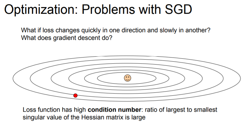
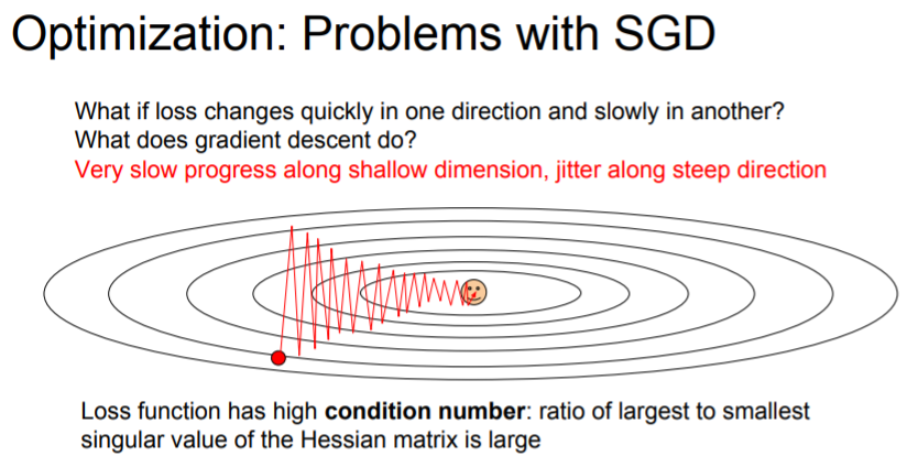
The direction of gradient does not align with the direction towards the minima. In effect, you get very slow progress along the horizontal dimension. This is undesirable behavior. This problem is more common in high dimensions.
(2) Local minima
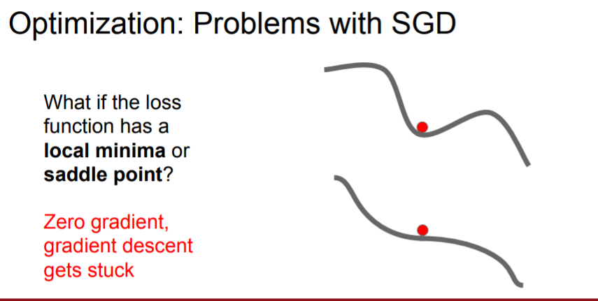
The function will get stuck at the saddle point(or near saddle point) because the gradient is zero! This is more common in high dimension, too.
(3) Stochastic problem
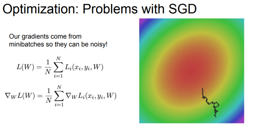
If there's noise in your gradient estimates, then vanilla SGD meanders around the space and might take a long time to get towards the minima.****
SGD + Momentum
Now we talked about the problems, and there's a simple strategy. The idea is about adding momentum term in SGD.
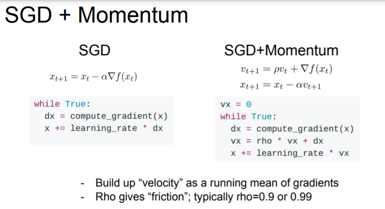
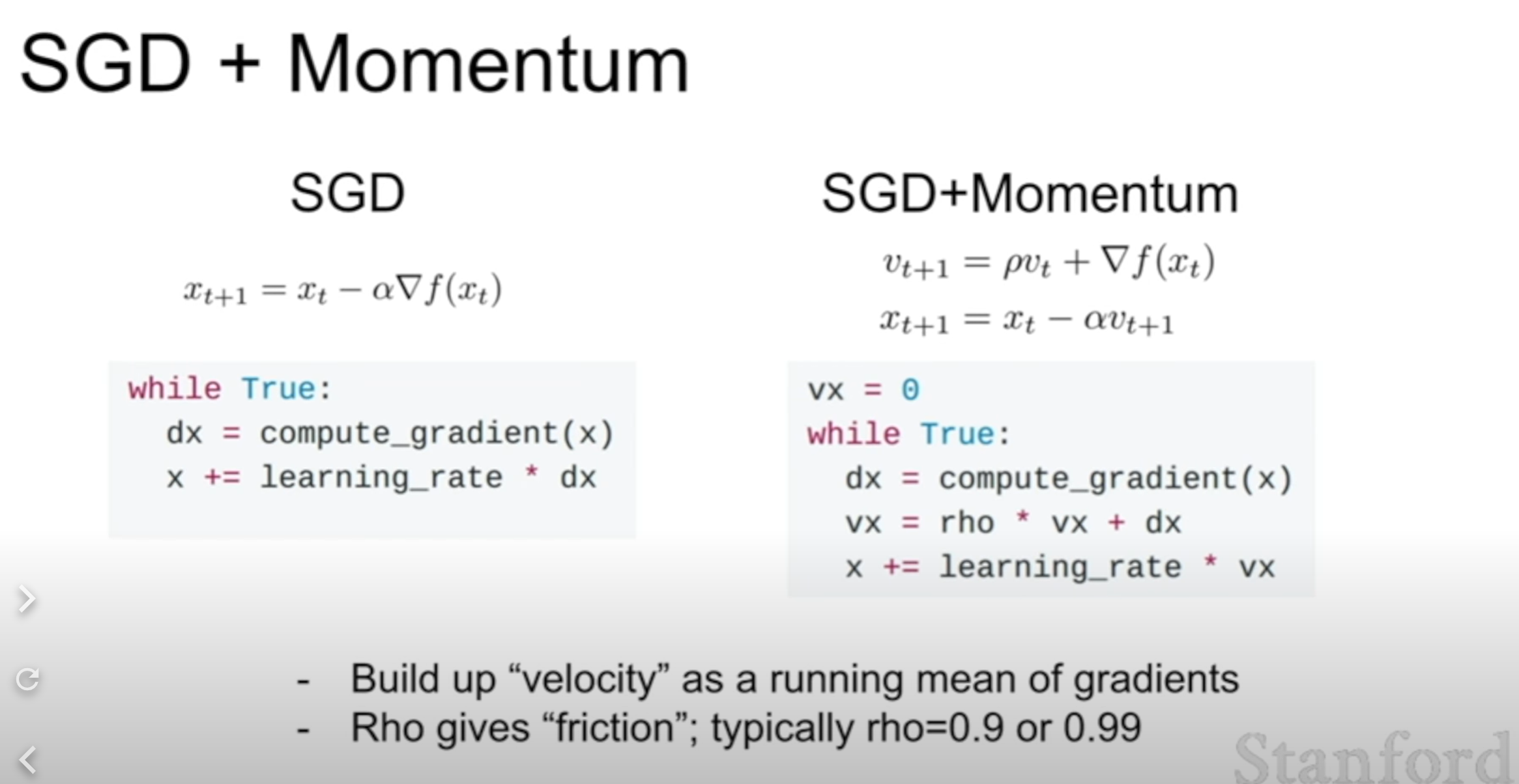
We maintain a velocity over time, and we add out gradient estimates to the velocity. Then we step in the direction of the velocity, rather than of the gradient.
We also have hyperparameter which corresponds to friction.(common choice: 0.9)
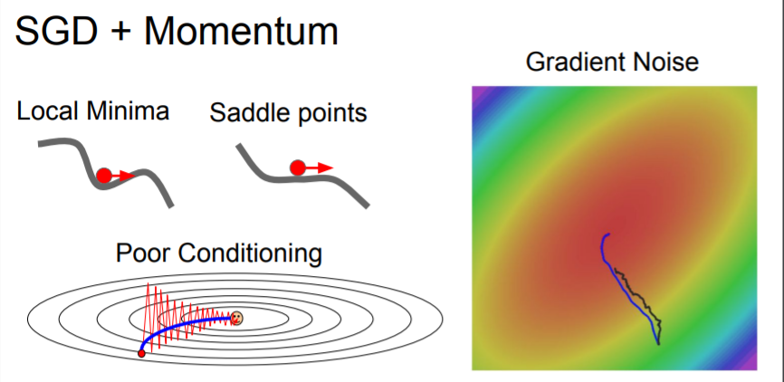
Adding momentum can get over Local minima problem and dealing with high condition number problem.
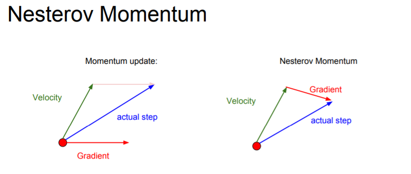
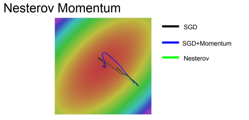
When we use Nesterov accelerated gradient, you step in the direction of where the velocity would take you and after that, evaluate the gradient at that point. You can imagine that you mix them a little more.
AdaGrad
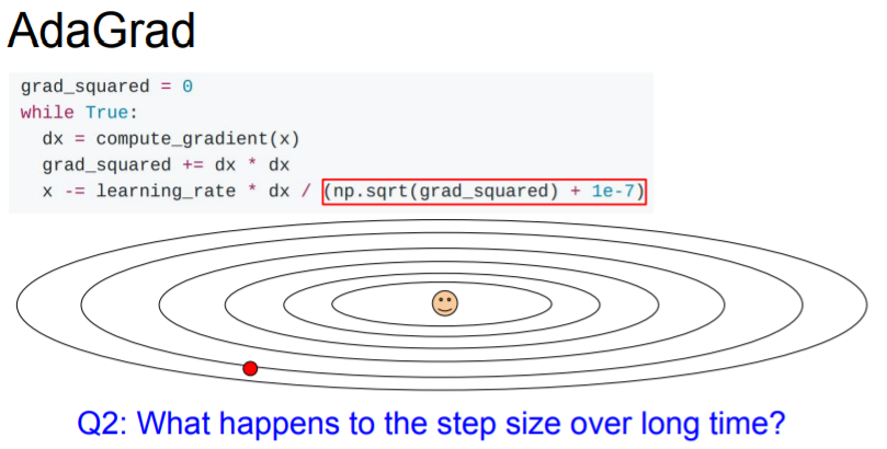
The idea with AdaGrad is that you're going to keep a running estimate or running sum of all squared gradients that you see during training. Rather than having a velocity term, instead we have this grad squared term.
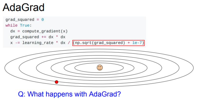
During the training, we are going to keep adding the squared gradients to this grad squared term. And when we update parameters, we divide by this grad squared term.
❔ What happens with AdaGrad over the course of training?
❕ The steps get smaller and smaller because we just continue to update the squared gradients over time, so we just grows and grows monotonically
RMSProp
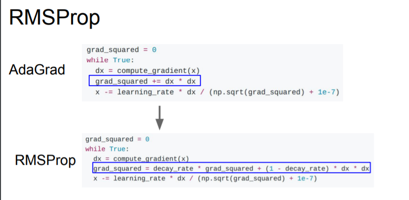
Now with RMSProp, we still keep this estimate of the squared gradients, but instead of letting that squared estimate continually accumulate over training, we let that squared estimate actually decay.
After we compute gradients with RMSProp, we take our current estimate of the grad squared and play it by this decay rate.
Because these are leaky, it addresses the problem of slowing down where you might don't want to.
What is leaky?
Question
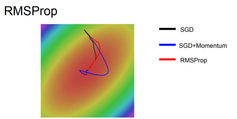
You can see that both of SGD+Momentum and RMSProp are better than vanilla SGD. However, SGD momentum, it overshoots the minimum and comes back, whereas with RMSProp, it's kind of adjusting its trajectory such that we're making approximately equal progress among all the dimensions.
So in momentum, we had this idea of velocity by adding in the gradients, and then stepping in the direction of the velocity. Also, we saw with AdaGrad and RMSProp that we gad this other idea of building up an estimate of squared gradients and then deciding by the squared gradients.
Why don't we just stick'em together?
That brings us to this algorithm called Adam!
Adam
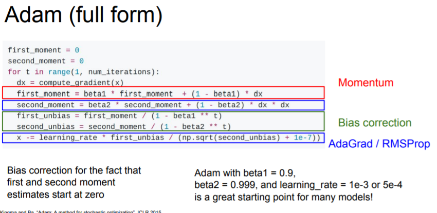
With Adam, we maintain an estimate of the first moment and the second moment. In the red, we make this first moment as a weighted sum of our gradients. And we have this moving estimate of the second moment like AdaGrad and RMSProp, which is a moving estimate of our squared gradients.
At update step, we use both the first moment, which is kind of our velocity, and also divide by the second moment, which is this squared gradient term.
It incorporates the nice properties of both. But there's a little of a problem here. What happens at the very first time step?
You can see that at the first time of beginning, we've set initialized our second moment with zero. After one update of the second moment, typically this beta two, second moment decay rate, is like 0.9 or 0.99. So after one update, our second_moment is still very close to zero.
Now when we're making our update step here, and we divide by our second moment, now we're diving by a very small number. So we're making a very, very large step at the beginning. So this very large step at the beginning is not due to the geometry of the problem. It's an artifact of the fact that we initialized our second moment estimate was zero.
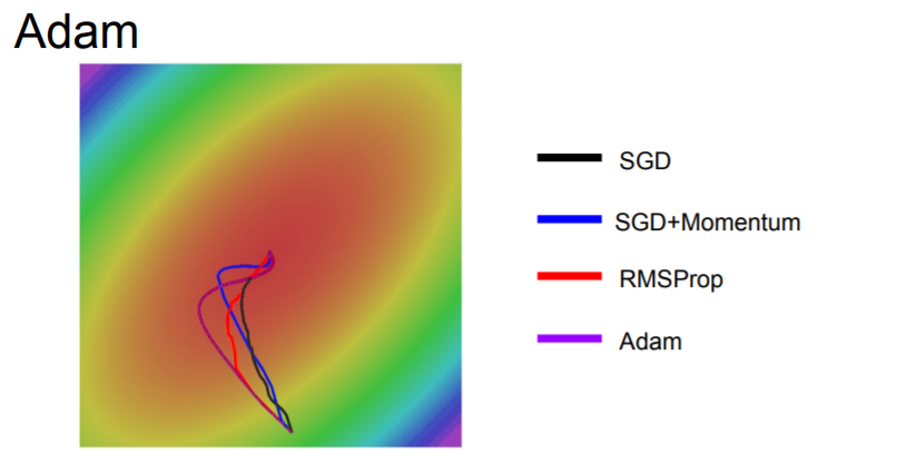
We can see that Adam overshoots the minimum a little, but it doesn't overshoot as much as momentum. Also, Adam has similar behavior of RMSProp of kind of trying to curve to make equal progress along all dimensions.
First-Order Optimization
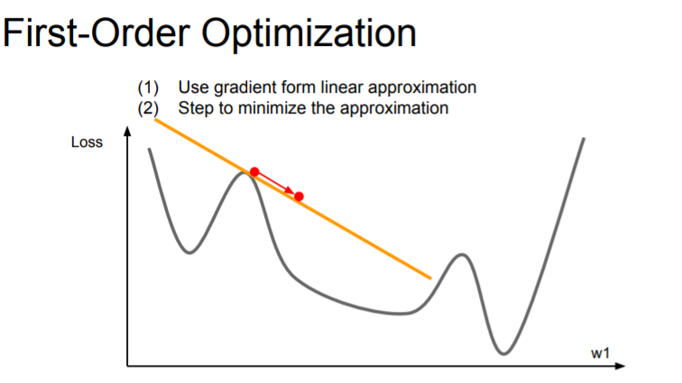
We're using the gradient information to compute a first-order of Taylor approximation to our function. But this approximation doesn't hold for very large regions, so we can't stop too far in that direction.
Second-Order Optimization
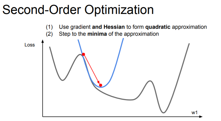
Actually you can go a little bit fancier. There's this idea of second-order approximation. We take into account both first derivative and second derivative information.
Now we make a second-order Taylor approximation to our function and kind of locally approximate our function with a quadratic.
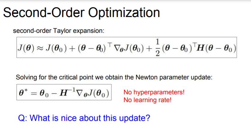
This doesn't have a learning rate in vanilla version!
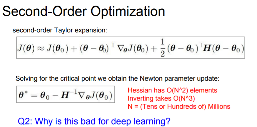
But this might be impractical for deep learning because this Hessian matrix is N by N(N=number of parameters). If N is a million, then the Hessian matrix is 1 million squared and this is too big.
2. Regularization
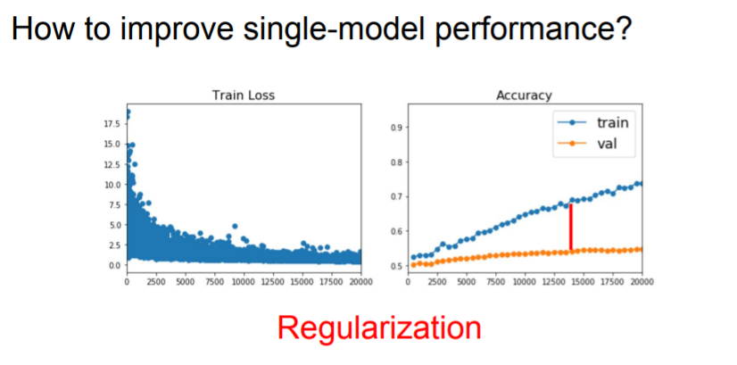
And you might get a question about how can we actually improve the performance of single models?
That's really this idea of regularization, where we add something to our model, to prevent it from fitting the training data too well and to make our model to perform better on unseen data.
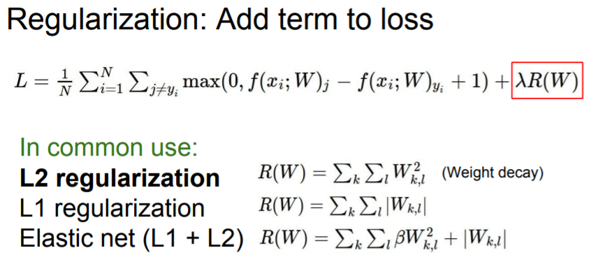
As we said before, L2 regularization doesn't really make a lot of sense in the context of neural networks. So sometimes we use other thing for neural networks.
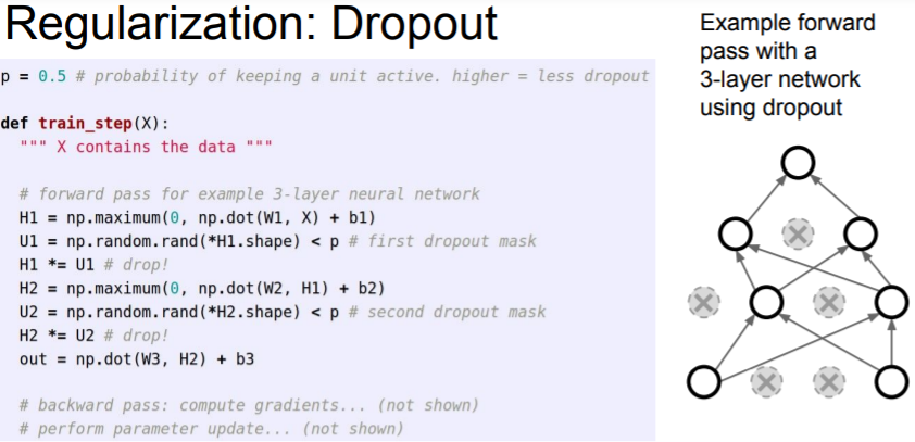
One regularization strategy is Dropout. You can see that after we do dropout, it looks like a smaller version of the same network where we're only using some subset of the neurons. This subset we use varies at each iteration.
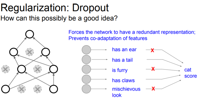
So the question is that why is it a good idea?
One sort of slightly hand wavy idea is that dropout helps prevent co-adapation of features.
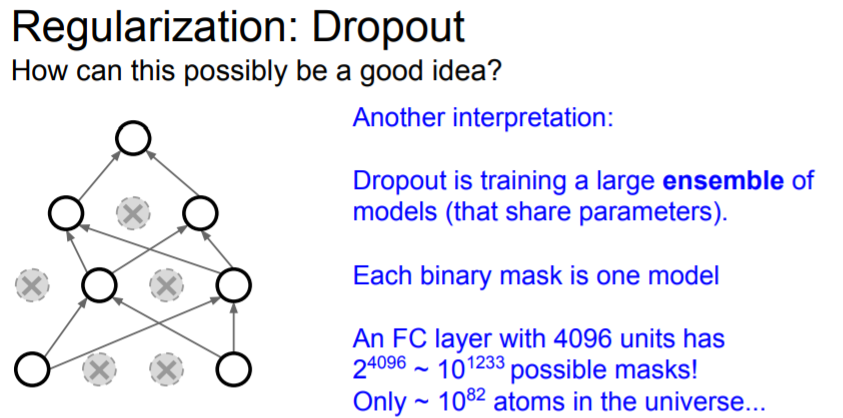
Another interpretation that's come out recently is that it's kind of like doing model ensembling within a single model. Every different potential dropout mask leads to a different potential subnetwork.
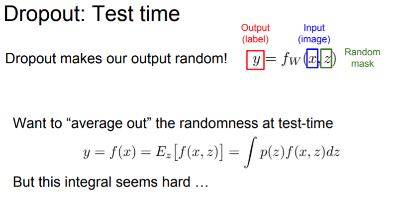
Then what happens at test time?
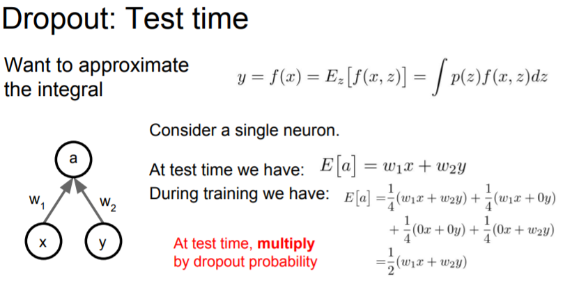
At test time, we don't have any stochasticity. Instead, we just multiply this output by the dropout probability.
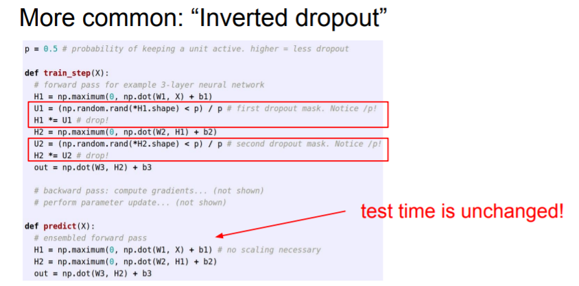
At test time, we usually use the entire weight matrix without multiplying p, but at training time, instead you divide by p because training is probably happening on a GPU. So you don't have to care if you do one extra multiply at training time. But at test time, you want this thing to be as efficient as possible.
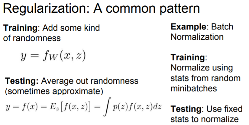
Where during training, we add some randomness to the network to prevent it from overfitting. Now at test time, we want to average out all that randomness to improve our generalization.
3. Transfer Learning
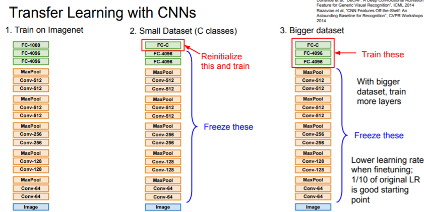
We've seen with regularization, we can reduce the gap between train and test error by adding these different regularization strategies.
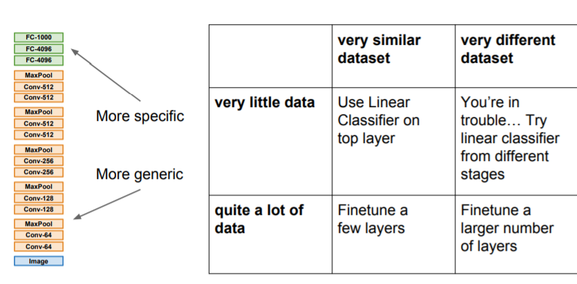
One problem with overfitting is that sometimes you don't have enough data. A big, powerful model can be overfitted too much on your small dataset.
4. Summary
