NumPy - (N, )과 1D Array의 Dot product, 그리고 Broadcasting

(N, )

"도대체 왜 이렇게 적혀있을까?" 라고 생각이 드는 1D Array의 shape 표기법...
일단 중요한 것은

1. (N, ) 는 1차원 Array이다.
2. (N, ) 는 (1,N), (N,1) 과 같지 않다.
   +. (1,N), (N,1) 들은 2차원 Array이다.

아래의 예시를 봐보자

ex) (N, )

A = np.arange(6)
print(A)
print(A.shape)

[0 1 2 3 4 5]
(6,)

---

ex) (1,N)

A_2D_1 = A.reshape(1,6)
print(A_2D_1)
print(A_2D_1.shape)

[[0 1 2 3 4 5]]
(1, 6)

대괄호가 두겹으로 된거보이지?

---

ex) (N,1)

A_2D_2 = A.reshape(-1,1)
print(A_2D_2)
print(A_2D_2.shape)

[[0]
 [1]
 [2]
 [3]
 [4]
 [5]]
(6, 1)

[+] Tips : A.reshape(-1,1)에서 -1의 의미는 "알아서 맞춰라" 라는 뜻이다. 즉 A 안의 요소개수는 6개이다. 이 A로 만들 수 있는 ( r,1 ) 배열은 무엇일까? r = 6
만약 A.reshape(-1,2)이라고 하면 r = 3이 되므로 (3,2) Array를 반환한다.
열위치에서도 마찬가지이다. A.reshape(2,-1)이라고 하면 c = 3이므로 (2,3) Array를 반환한다.

---

일단
1차원 Array인 (N, )이
2차원 Array인 (1,N), (N,1)와 다르다는 점은 알았다.

이제 1차원 Array의 행렬곱, 즉 Dot product, 내적에 대해서 알아보자

---

1차원 Array의 Dot product, 내적, 행렬곱

Keypoint :
(N, ) 1차원 Array가 앞에있으면 가로 짝대기 (1,N) 1행으로, 뒤에있으면 세로 짝대기 (N,1) 1열로 생각하자

A = np.array( [1, 2, 3] )
B = np.array( [4, 5, 6] )
np.dot( A,B )

32

$\color{red}\begin{pmatrix} 1 & 2& 3 \end{pmatrix}$ $\cdot$ $\color{blue}\begin{pmatrix} 4 \\ 5 \\ 6 \end{pmatrix}$ $= (1\times4) +(2\times5)+(3\times6)=4+10+18=32$

즉...
(3, ) $\cdot$ (3, ) 의 행렬곱이
(1,3) $\cdot$ (3,1) 처럼 되면서
=(1,1)로됨
근데 1차원 Array끼리의 행렬곱은 0차원이 되어야 하므로 ( , ) 즉 Scalar값이 됨!

---

X = np.arange(1,7).reshape(2,3)
print(X)
print(X.shape)

[[1 2 3]
 [4 5 6]]
(2, 3)

ones_2 = np.ones(2)
ones_3 = np.ones(3)
print(ones_2)
print(ones_2.shape)
print("---------")
print(ones_3)
print(ones_3.shape)

[1. 1.]
(2,)
---------
[1. 1. 1.]
(3,)

자 X는 (2,3) 2차원 행렬이고
ones_2는 (2,) 1차원 행렬
ones_3은 (3,) 1차원 행렬

---

np.dot( ones_2, X)

array([5, 7, 9])

$\begin{pmatrix} 1&1 \end{pmatrix}$ $\cdot$ $\begin{pmatrix} 1&2&3 \\ 4&5&6 \end{pmatrix}$
$=[(1\times1+1\times4),\;\; (1\times2+1\times5),\;\;(1\times3+1\times6)]$
$=[5,7,9]$

즉...
(2, ) $\cdot$ (2,3) 의 행렬곱이
(1,2) $\cdot$ (2,3) 처럼 되면서
=(1,3)로 됨
근데 1차원 Array랑 곱하면 1차원이 되어야하므로... (3, )이 되는거임

---

np.dot( X, ones_3)

array([ 6, 15])

이번엔 행렬곱 연산의 결과물의 Shape이 무엇인지 맞혀보자
(2,3) $\cdot$ (3, ) 의 행렬곱이
(2,3) $\cdot$ (3,1) 처럼 되면서
=(2,1)로 됨
근데 1차원 Array랑 곱하면 1차원이 되어야하므로... (2, )이 되는거임

$\begin{pmatrix} 1&2&3 \\ 4&5&6 \end{pmatrix}$ $\cdot$ $\begin{pmatrix} 1\\1\\1 \end{pmatrix}$

$=[(1\times1+2\times1+3\times1), \;\;\; (4\times1+5\times1+6\times1)]$
$=[6, \;15]$

---

Broadcasting

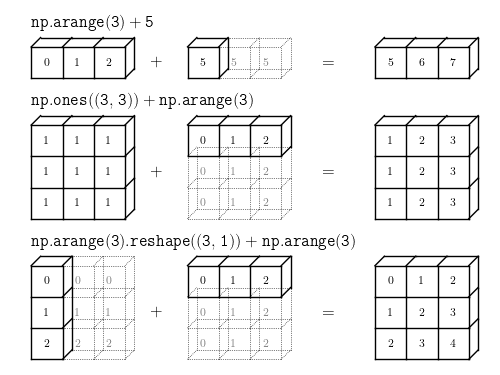
출처 : http://www.astroml.org/book_figures/appendix/fig_broadcast_visual.html
출처 : https://sacko.tistory.com/16 [데이터 분석하는 문과생, 싸코]

[+] broadcast : v. 퍼뜨리다, adj. 널리 퍼져 있는

Keypoint :
matrix간의 연산은 원래 shape가 같아야지 연산이 가능하다.
왜냐하면 element-wise operation(Hadamard operation?), 즉 각 matrix의 같은 위치의 요소끼리의 연산이므로...

M = np.arange(1,10).reshape(3,3)
print(M)
print(M.shape)

print("-----------")
N = np.array(1)
print(N)
print(N.shape)

[[1 2 3]
 [4 5 6]
 [7 8 9]]
(3, 3)
-----------
1
()

print(M+N)
print(M*N)

[[ 2  3  4]
 [ 5  6  7]
 [ 8  9 10]]
[[1 2 3]
 [4 5 6]
 [7 8 9]]

그런데 위,아래와 같이 (3,3) Matrix와 () Matrix를 더하고 곱하면
M행렬의 각 요소에 N행렬의 요소를 알아서 더하고 곱해준다.
이거를 그냥 NumPy Array 연산의 편리함이라고 생각했으나 이게 바로 Broadcasting 개념이라고 볼 수 있다.