[PyTorch] Autograd-02 : With Jacobian

olxtar·2022년 3월 30일

DeepLearning PyTorch math

[PyTorch] Autograd

목록 보기

2/5

-> [PyTorch] Autograd-02. With Jacobian
에 이어서 작성...

0. Autograd

왜왜왜 .backward() 앞이 loss Scalar Tensor일때는 되고(~여야하고)
왜왜왜 .backward(gradient tensor)는 되는걸까

$\cdots$
일반적으로 손실함수 (loss function)을 계산할 때는 배치에 대하여 평균/합 등을 통해 스칼라 값을 만들어준 이후에 .backward() 함수를 적용합니다. Scalar Loss에 대한 각 parameter별 gradient를 계산하고 최적화를 수행.
$\cdots$

출처 : https://hongl.tistory.com/273

PyTorch에서는 JVP(Jacobian Vector Product) 를 계산하여! 즉 통하여 최종 parameter(weight)에 대한 loss의 gradient를 계산함! $\rightarrow$ 그래서 어떻게? JVP가 뭐야 ㅠㅠ

1. Loss와 Loss Function

1-1. Loss

먼저 Loss에 대해서 조금 짚고 넘어가자.
0~9까지의 숫자 손글씨를 분류하는 Image classification 같은 경우에
단 1 개의 Image를 input으로 넣었을 때, output layer's node에서는 0~9까지 즉, 10개의 output 값이 나온다.

(\hat{y_0},\hat{y_1},\cdots,\hat{y_9})

그리고 우리는 그 단 1 개의 Image가 무슨 숫자인지 즉, 정답(label,target)을 알고있다. 이는 당연히 아래와 같이 나타낼 수 있다. 예를들어서 정답이 숫자 '9'일 경우...
(0=False, 1=True) 느낌

(0,0,\cdots,1)=(y_0,y_1,\cdots,y_9)

이러한 상황에서, 단 1 개의 Image에 대하여 model이 예측한 값(들) $\hat{y}$ 의 Loss는 (다양하게 정의되지만 편하게, 보통,) $y$ 와 $\hat{y}$ 가 얼마나 다르냐! 가 바로 Loss의 개념이다.

여기서 Keypoint는
단 1 개의 Image에 대한 모든 output값과 정답과 얼마냐 다르냐!인 Loss를 보통...하나의 값으로 만든다. 이다.

Loss =[(y_0-\hat{y_0})+(y_1-\hat{y_1})+\cdots+(y_9-\hat{y_9})]=\displaystyle\sum_{i=0}^9(y_i-\hat{y_i})

10개의 output $y$ 와 target $\hat{y}$ 를 Tensor로 나타내면
즉, $y_{tensor}$ 와 $\hat{y}_{tensor}$ 를 (1,10)의 size를 가진 Tensor(2D vector)라고 생각하면... 위 수식이 아래와 같이 표현된다.
(여기서 숫자 1은 input의 개수, 10은 output layer's node의 개수, Class의 개수)

Loss=\sum y_{tensor}-\hat{y}_{tensor}

1. 저 Sigma는 Tensor의 모든 요소를 더하는거라 생각하면 된다.(Tensor끼리의 단순 연산의 결과는 같은 사이즈의 Tensor!)

2. 단 하나의 input에 대해서 단 하나의 loss가 나온다는거만 기억하자. 이 Loss는 단순개념적으로 풀어쓴것임. 절~대 이런게 아님 -> MSE, CrossEntropy

1-2. Loss Function

PyTorch와 같은 DeepLearning관련 프레임워크에서의 Loss function은 거의다(?) batch단위의 input을 받는다. 아니 받을것이다...
(input 한개 한개 받아서 loss구해서 Gradient Descent Step밟으면...언제 다해...)

예를 들어서 아래와 같은 Code가 있다하면...

# The number of input data : 64000
# train_loader's batch_size=64

n_epochs = 100
for epochs in range(n_epochs):                  # epochs loop
	train_loss = 0.0
    
    for data, target in train_loader:           # batch loop
    	...
        output = model(data)
        loss = criterion(output, target)
        loss.backward()
        optimizer.step()
        
        train_loss += loss.item()
        
     train_loss = train_loss/len(train_loader)

지금 위와 같은 # batch loop를 통해서 loss값이 train_loss에 누적되었지?
그러면 전체 데이터를 한번 다 훑은 즉, 1 epoch의 진짜 train_loss는 무엇일까?

내가 가진 data의 개수가 64,000개 / batch_size=64
그러면 DataLoader는 총 몇개의 Batch를 뱉을까?
$\rightarrow$ 64,000 $\div$ 64 $=$ 10,000
Tip : len(DataLoader) : DataLoader가 뱉는 batch 개수!

$\rightarrow$ train_loss = train_loss/len(train_loader)
위와 같이 1 epoch동안 누적된 10,000개의 loss값이므로 len(train_loader)로 나눠줘야한다.

[+] 이렇게 해도 된다!

for epoch~                                   # epoch loop
	...
	for data, target in train_loader:        # batch loop
		...
		train_loss += loss.item() * data.size(0)
	...
	train_loss = train_loss / len(train_loader.dataset)

data : DataLoader, 즉 train_loader로 받은 1개의 batch, 따라서 data.size(0)은 batch 덩어리의 Row shape이므로 batch size가 된다.(=64)
즉, loss.item()*data.size(0)은 loss function이 기껏 구한 loss값에다가 다시 batch size를 곱해서 한번의 batch에서의 각 input data들의 loss의 총합이다.

len(train_loader.dataset) : 이렇게하면 train_loader가 가지고 있는 진짜 데이터의 수를 반환한다. (=64000)

2. Jacobian Matrix and Jacobian Vector Product

2-1. Jacobian Matrix (J)

참고 : [편미분을 간단하게! - Jacobian Matrix]
참고 : https://towardsdatascience.com/pytorch-autograd-understanding-the-heart-of-pytorchs-magic-2686cd94ec95

Mathmatically, the autograd class is just a Jacobian-Vector Product computing engine. A Jacobian matrix in very simple words is a matrix representing all the possible partial derivatives of two vectors. It's the gradient of a vector with respect to another vector.
PyTorch의 Autograd Class는 수학적으로 말하자면, 야코비안 벡터 프로덕트를 계산하는 엔진이다.
야코비안 매트릭스를 단순히 말하자면, 두 벡터 사이 가능한 모든 편미분을 나타내는 행렬이다.
다시 말하자면, 다른 Vector에 대한 어떤 Vector의 Gradient이다.

ex) Jacobian-Matrix

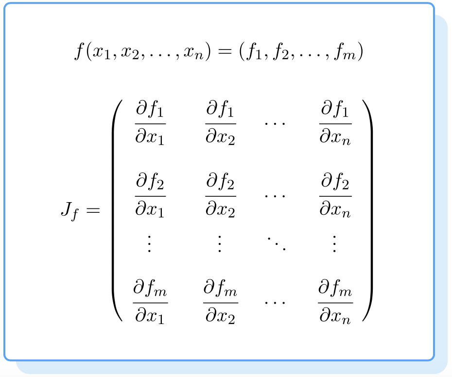
만약 하나의 함수가 n개의 변수를 가지고 있다고 가정해봅시다.
그리고 그런 함수가 m개 있음.

F_1(x_1,\dots,x_n)

F_2(x_1,\dots,x_n)

\dots

F_m(x_1,\dots,x_n)

위와 같은 함수들의 편미분하려면 아래 J 와 같은 벡터로 표현한다. 이것이 바로 Jacobian Matrix

J=\begin{bmatrix} \frac{\partial F_1}{\partial x_1} & \cdots & \frac{\partial F_1}{\partial x_n} \\ \vdots & \ddots & \vdots \\ \frac{\partial F_m}{\partial x_1} & \cdots & \frac{\partial F_m}{\partial x_n} \end{bmatrix}

\;\;\;\;\;\;\;\;size=(n \times m) \;\;J \;vector

2-2. Jacobian Vector Product (JVP)

$X=[x_1,x_2,\cdots,x_n]$ (Let this be the weights of some machine learning model)

$X$ undergoes some operations to from a vector $Y$

$Y=f(X)=[y_1,y_2,\cdots,y_m]$

$Y$ is then used to calculate a scalar loss $l$ . Suppose a vector $v$ happens to be the gradient of the scalar loss $l$ with respect the vector $Y$ as follows

v=\left(\frac{\partial l}{\partial y_1}\;\;\;\cdots\;\;\;\frac{\partial l}{\partial y_m}\right)^T

loss값을 각 output value, y1,y2...ym에 대하여 편미분이라...

The $vector \;v$ is called the grad_tensor and passed to the backward() function as an argument.

Jacobian Vector Product

To get the gradient of the loss $l$ with respect to the weights $X$ ,
The Jacobian matrix $J$ is vector-multiplied with the $vector\; v$

\frac{\partial loss}{\partial X}=J_{(XY)}\cdot v

즉 X vecotr에 대한 loss의 편미분값을 구하려면 X,Y vector의 Jacobian Matrix와 위에서 설명한 v vector를 벡터곱 해줘야한다(?)

$J$ : Jacobian matrix with $X\; vector$ and $Y\;vector$

J=\begin{bmatrix} \frac{\partial y_1}{\partial x_1} & \cdots & \frac{\partial y_m}{\partial x_1} \\ \vdots & \ddots & \vdots \\ \frac{\partial y_1}{\partial x_n} & \cdots & \frac{\partial y_m}{\partial x_n} \end{bmatrix}

$v$ : Gradient Tensor of the scalar loss $l$ with respect the $Y\;vector$

v=\left(\frac{\partial l}{\partial y_1}\;\;\;\cdots\;\;\;\frac{\partial l}{\partial y_m}\right)^T

$J\cdot v$

J\cdot v=\begin{pmatrix} \frac{\partial y_1}{\partial x_1} & \cdots & \frac{\partial y_m}{\partial x_1} \\ \vdots & \ddots & \vdots \\ \frac{\partial y_1}{\partial x_n} & \cdots & \frac{\partial y_m}{\partial x_n} \end{pmatrix} \begin{pmatrix}\frac{\partial l}{\partial y_1} \\ \vdots \\ \frac{\partial l}{\partial y_m}\end{pmatrix}= \begin{pmatrix}\frac{\partial l}{\partial x_1} \\ \vdots \\ \frac{\partial l}{\partial x_n}\end{pmatrix}

This method of calculating the Jacobian matrix and multiplying it with a $vector\;v$ enables the possibility for PyTorch to feed external gradients with ease for even the non-scalar outputs.
야코비안 행렬을 계산하고
vector v로 곱하는 이 방법은
non-scalar 출력에 대해서도 쉽게 외부 Gradient를 공급할 수 있게끔한다(?)

[?] non-scalar에 대한 .backward()에서 external gradient는 무엇을 줘야되고 어떻게 계산되는가?

잠깐만...

loss_scalar.backward()
loss_vector.backward(external_gradient) = loss_vector.backward(v)

원래 .backward() 함수는

?????????????????????????????????헷갈령

3. 다시 Autograd

참고 : https://hongl.tistory.com/273
참고 : https://towardsdatascience.com/pytorch-autograd-understanding-the-heart-of-pytorchs-magic-2686cd94ec95

3-1. PyTorch Tensor and Dynamic Computation Graph (DCG)

Tensor: In simple words, its just an n-dimensional array in PyTorch.
DCG (Dynamic Computation Graph): On setting .requires_grad=True they start forming a backward graph that tracks every operation applied on them to calculate the gradients using something called a dynamic computation graph (DCG)
.requires_grad=True를 가진 Tensor는... 해당 Tensor에 적용되는 모든 연산을 트래킹한다. Gradient를 계산하기 위해서!

# Tensor 생성 및 Turn requires_grad on
a = torch.randn(2,2, requires_grad=True)
print(a)

>>
tensor([[0.5818, 2.1532],
        [1.1036, 0.8144]], requires_grad=True)

-------------------------------
# Turn requires_grad off
a.requires_grad_(False)
print(a)

>>
tensor([[0.5818, 2.1532],
        [1.1036, 0.8144]])
        
        
-------------------------------
# From NumPy
b = np.array([1.,2.,3.])    #Only Tensors of floating point dtype can require gradients
b = torch.from_numpy(b)
b.requires_grad_(True)
print(b)

>>
tensor([1., 2., 3.], dtype=torch.float64, requires_grad=True)

3-2. Autograd and Backpropagation

[+] acyclic : adj. 비순환적인

Autograd: This class is an engine to calculate derivatives (Jacobian-vector product to be more precise). It records a graph of all the operations performed on a gradient enabled tensor and creates an acyclic graph called the dynamic computational graph.
Autograd Class는 도함수를 계산하기 위한 Engine이다.
Autograd는 Tensor에 적용된 모든 연산을 기록하여 비순환적인 graph를 그린다.

The leaves of this graph are input tensors and the roots are output tensors. Gradients are calculated by tracing the graph from the root to the leaf and multiplying every gradient in the way using the chain rule.
leaf = input tensor
root = output tensor
From root to leaf 즉, 뿌리에서 잎까지 체인룰을 이용하여 모든 Gradient를 곱하면서 최종(?) Gradient를 구한다.

[+] composite : n. 합성물, adj. 합성의
[+] from scratch : from the very beginning or starting point. from nothing

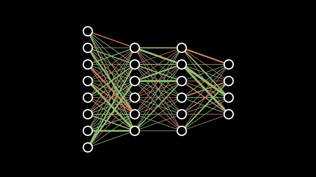
Backpropagation: Neural networks are nothing more than composite mathmatical function that are delicately tweaked (trained) to output the required result. The tweaking or the training is done through a remarkable algorithm called backpropagation. Backpropagation is used to calculate the gradients of the loss w.r.t. the input weights to later update the weights and eventually reduce the loss.
Neural Network는 Output을 원하는 값으로 만들기 위한 수학적 함수의 합성물이다.
Backpropagation은 아래 수식과 같이 The Gradient loss with respect to input weight를 계산하는 것! $\frac{\partial loss}{\partial w}$

The change in the loss for a small change in an input weight is called the gradient of that weight and is calculated using backpropagation. The gradient is then used to update the weight using a learning rate to overall reduce the loss and train the neural net.
input weight의 변화에 대한 loss의 변화...

This is done in an iterative way.
$\cdots$
PyTorch does it by building a Dynamic Computational Graph (DCG). This graph is built from scratch in every iteration providing maximum flexibility to gradient calculation.
매 iteration마다 graph를 새롭게 그린다...

3-3. About the DCG

Dynamic Computational Graph (DCG): Gradient enabled tensors (variables) along with functions (operations) combine to create the dynamic computational graph. The flow of data and the operations applied to the data are defined at runtime hence constructing the computational graph dynamically.
Variable 즉, requires_grad=True인 Tensor와 / Operation 즉, function들로 DCG를 그린다.
Data의 흐름과 연산은 Autograd Class에 의하여 동적으로 즉, 바로바로~ Graph화 된다.

requires_grad=False

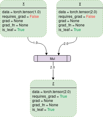
Variable: 초록색 네모박스
Operation: 보라색 네모박스
Data: It's the data a variable is holding.

$x$ 는 (1x1) 사이즈의 1.0

$y$ 는 (1x1) 사이즈의 2.0

$z$ 는 (1x1) 사이즈의 2.0

requires_grad: If 'true' starts tracking all the operation history and forms a backward graph for gradient calculation.
grad: grad holds the value of gradient. False일때는 당연히 아무 값도 없음. True이고 다른 node(Variable)에서 .backward()를 호출하여야지 값을 가짐.

ex) Variable $x$ 를 가진 즉, $x$ 를 연산한 Variable $out$ 에 대해서 out.backward() 호출 시 x.grad()는 $\frac{\partial out}{\partial x}$ 값을 가짐!
grad_fn: This is the backward function used to calculate the gradient.

어떤 root node(output variable)에 대해서 .backward()를 호출하면
requires_grad와 is_leaf가 True인 leaf node(input variable)에 대하여 output을 편미분한 Gradient값이 각각의 leaf node에 생성된다.

※ 위 그림(DCG)는 requires_grad=False임!
※ 아래 그림(DCG)는 requries_grad=True임!

requires_grad=True

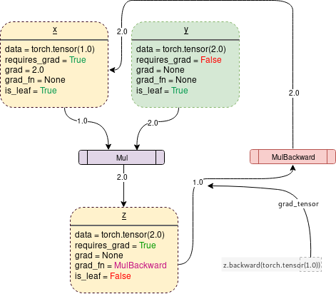
On turning requires_grad=True, PyTorch Autograd Engine will start tracking the operation and store the gradient functions at each step as follows
위 그림처럼 x의 requires_grad를 True로 해주면
z가 MulBackward 즉, Mul의 역방향 함수를 갖게된다(?).

3-4. Backward() function

Backward is the function which actually calculates the gradient by passing it's argument(1x1 unit tensor by default) through the backward graph all the way up to every leaf node traceable from the calling root tensor.
.backward()는 argument(함수가 받는 input값)를
backward function을 호출한 root로부터~
추적가능한 모~든 leaf node들에 통과시키면서 Gradient를 계산한다.

THe calculated gradients are then stored in .grad of every leaf node.
계산되는 gradient는 각 leaf node의 .grad에 저장된다

Remember, the backward graph is already made dynamically during the forward pass. Backward function only calculates the gradient using the already made graph and stores them in leaf nodes.
(requires_grad=True를 한 상태에서!) forward pass를 진행하면 자동으로 backward graph가 생성된다!
따라서 backward function은 그냥 backward graph를 통해서 gradient들을 계산하고 각 leaf node에 저장해주는 역할은 한다!

An important thing to notice is that when z.backward() is called, a tensor is automatically passed as z.backward(torch.tensor(1.)). The torch.tensor(1.0) is the external gradient provided to terminate the chain rule gradient multiplications. This external gradient is passed as the input to the MulBackward function to further calculate the gradient of $x$ .
그냥 .backward() without argument 호출 시 자동으로 1x1사이즈의 유닛 텐서가 argument로 전달된다.
이 1x1사이즈의 유닛 텐서 즉, 사이즈 1x1이고 값도 1인 텐서는 external gradient로 z에 저장되어 있는 MulBackward function의 input으로 들어간다.

\frac{\partial z}{\partial z}

The dimension of tensor passed into .backward() must be the same as the dimension of the tensor whose gradient is being calculated.
.backward()에 전달되는 argument 즉, external gradient는 backward를 호출한 Tensor와 size가 같아야한다.
따라서 loss와 같은 Scalar값에는 그냥 .backward()만 호출하여도 default argument가 unit tensor이므로 작동하게된다.