[Machine Learning/머신러닝] MLP model - Sequential

사람의 손 글씨로 적힌 숫자를 보고 숫자를 인식해내는 MLP 모델을 만들어보고자 한다.

• 개발 환경 : tensorflow에서 진행
• 데이터셋 : kaggle에서 제공되는 mnist.csv 파일 사용

데이터셋, 개발 환경은 이전 글과 동일하다. 하지만 이번에는 Sequential API 방법을 사용해볼 것이다.

데이터셋 처리

각 행은 하나의 손글씨 숫자 이미지이고 형식은 [label, pixel1, pixel2, ..., pixel784]와 같이 숫자와 그에 해당하는 각 픽셀의 밝기 값이 저장되어 있다. 우리는 라벨과 픽셀값을 분류해줘야 한다.

#train의 전체 행 저장+Y만 출력, 앞에 빼고 출력(X train)
Y_train, X_train = utils.to_categorical(train[:,0]), train[:,1:]

#test의 전체 행 중 Y만 출력, 앞에 Y빼고 저장
Y_test, X_test = utils.to_categorical(test[:,0]), test[:,1:]

#정규화
X_train = X_train / 255.0
X_test = X_test / 255.0

TensorFlow vs. Keras

TensorFlow

• 직접 계산 그래프 작성
• placeholder, Variable, matmul 등 모든 연산을 명시적으로 정의
• 초기화, 세션 실행 등 수동 관리

🔧 구조 (example)

• x, y_: 입력/정답 placeholder
• W1, b1, W2, b2, W3, b3: 3층 MLP (입력 → 히든1 → 히든2 → 출력)
• relu, softmax 활성화 함수
• cross_entropy: 손실 함수 (수식 직접 구현)
• GradientDescentOptimizer: 수동 설정
• sess.run(tf.global_variables_initializer()): 변수 초기화 수동 실행

Keras

필자는 이번 코드에서 Keras를 사용할 것이다.

• 모델 정의가 간결하고 직관적
• Sequential() + add(Dense(...))로 레이어 구성
• 학습, 예측, 평가를 한 줄로 수행 가능

🔧 구조 (example)

• Sequential()로 모델 생성
• Dense(hidden_1, activation='relu') 등으로 레이어 구성
• compile()에서 손실 함수와 옵티마이저 지정
• summary()로 전체 구조 확인

먼저 MLP 구조를 만들어준다.

mlp_model = Sequential()
mlp_model.add(Dense(512, activation='sigmoid', input_shape=(784,))) # 입력층
mlp_model.add(Dense(256, activation='sigmoid'))
mlp_model.add(Dense(10, activation='softmax')) # 출력층 (0~9)
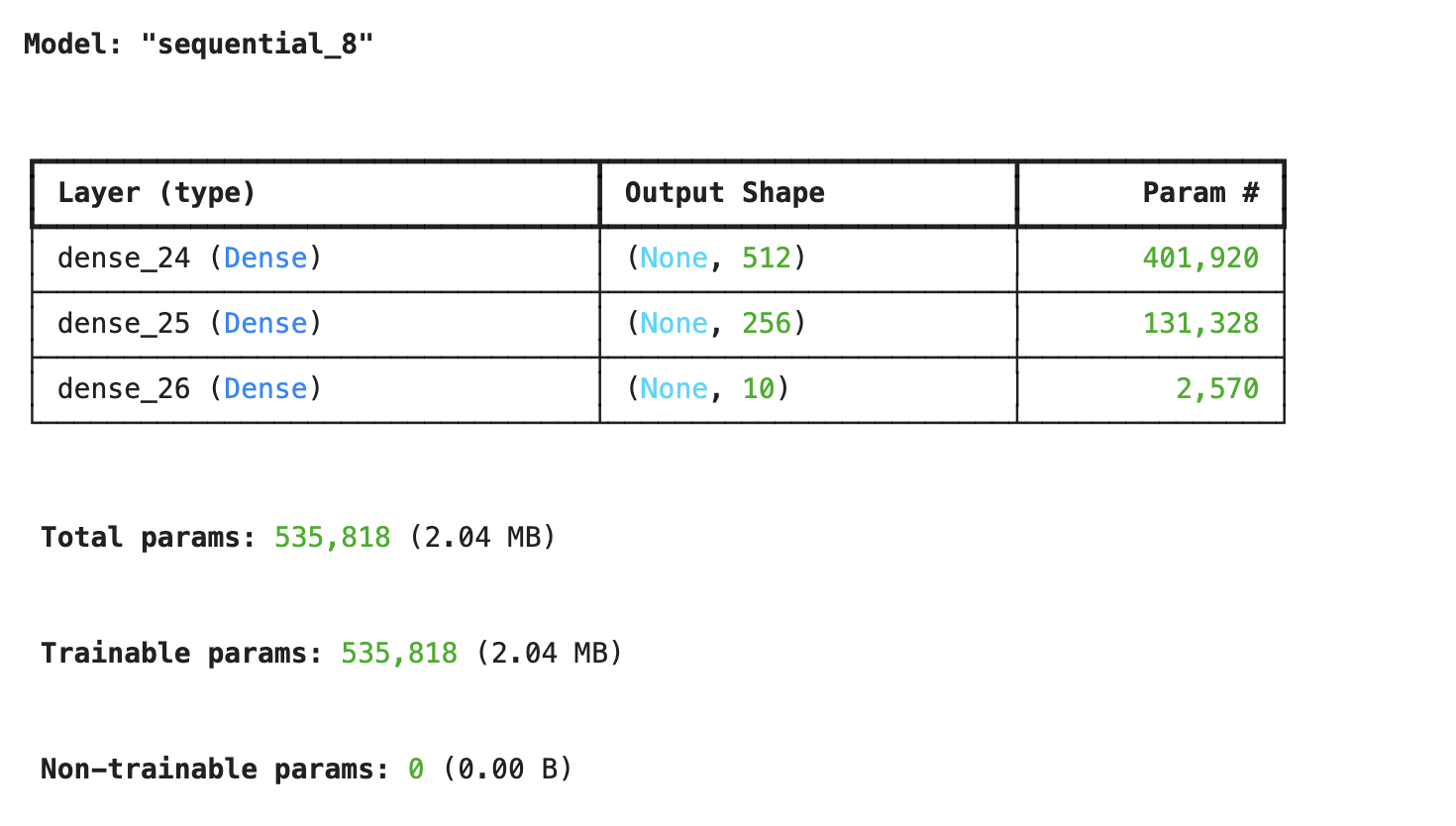
mlp_model.summary()

#sigmoid대신 relu 사용 가능

그럼 다음과 같이 학습 파라미터의 수가 시각적인 표와 함께 나온다.

relu vs. sigmoid

• relu : 학습이 빠르고 vanishing gradient 문제 없음
• sigmoid : 입력이 크면 gradient vanishing 발생. 간단한 MLP에서 잘 작동

학습/검증 데이터 정확도

mlp_model.compile(loss='categorical_crossentropy', optimizer='adam', metrics=['accuracy'])
model_history = mlp_model.fit(X_train, Y_train, validation_data=(X_test, Y_test),\
                            epochs=15, batch_size=512, shuffle=True, verbose=2)

다음과 같은 코드를 통해 학습/검증 데이터에 대한 정확도와 손실을 볼 수 있다.

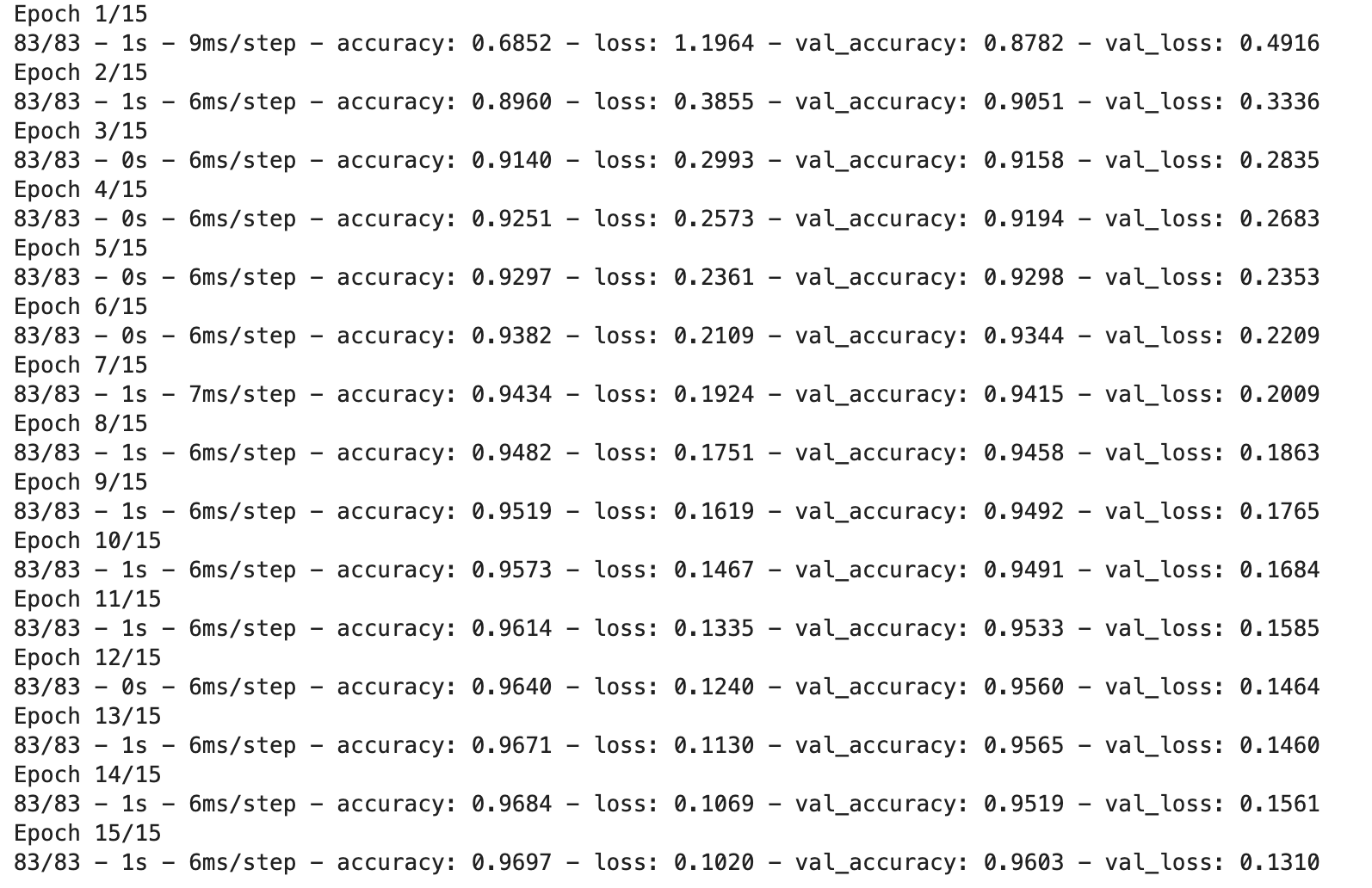
• 학습 정확도 : 96.97%
• 검증 정확도 : 96.03%

이후 정확도와 손실 그래프를 확인하기 위해 다음과 같이 시각화하였다.

정확도

import matplotlib.pyplot as plt

plt.plot(model_history.history['accuracy'])
plt.plot(model_history.history['val_accuracy'])
plt.title('model accuracy')
plt.ylabel('accuracy')
plt.xlabel('epoch')
plt.legend(['train', 'test'], loc='right')
plt.show()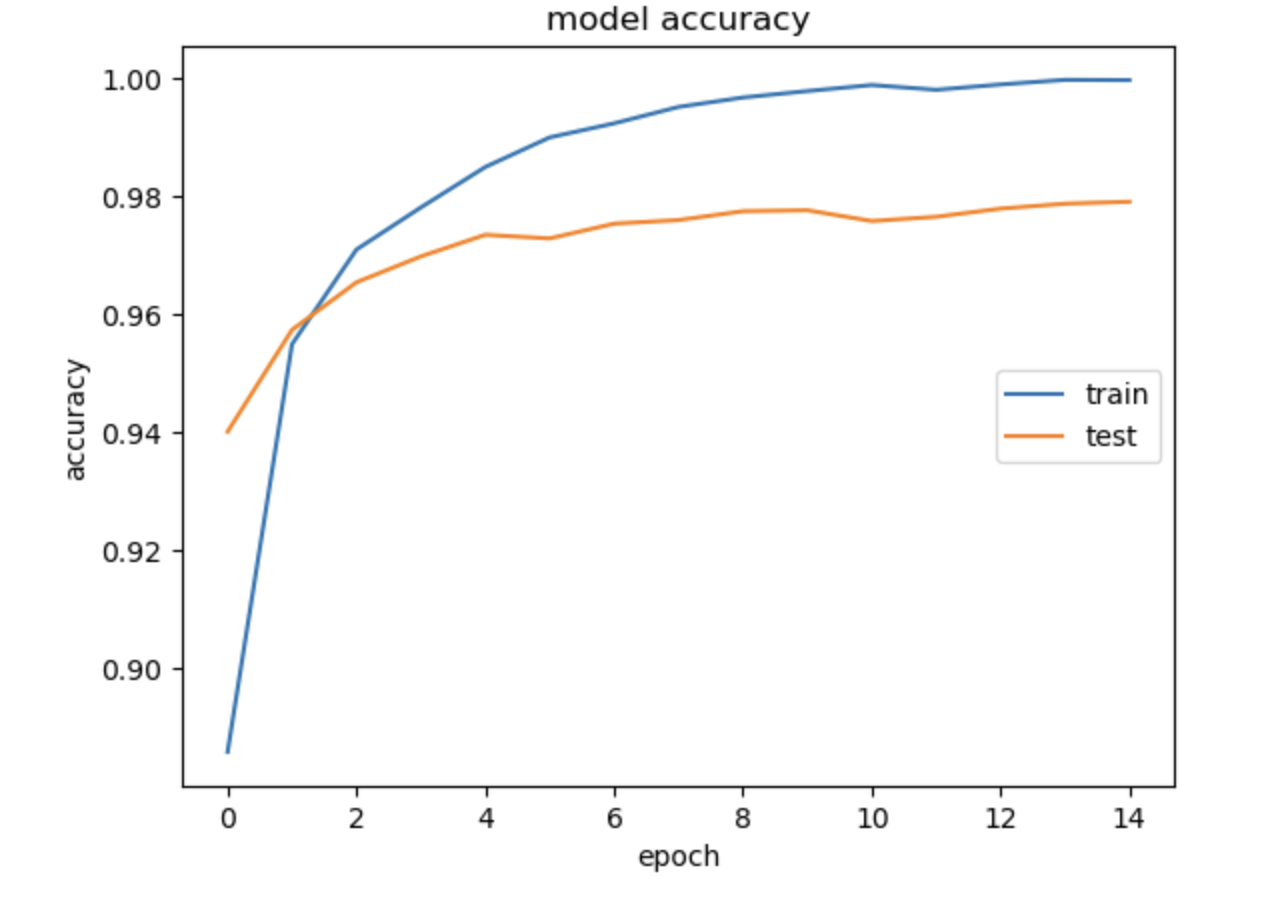

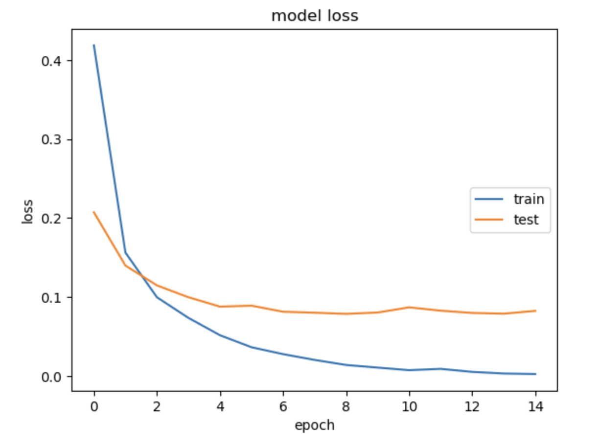
손실도

import matplotlib.pyplot as plt

plt.plot(model_history.history['loss'])
plt.plot(model_history.history['val_loss'])
plt.title('model loss')
plt.ylabel('loss')
plt.xlabel('epoch')
plt.legend(['train', 'test'], loc='right')
plt.show()

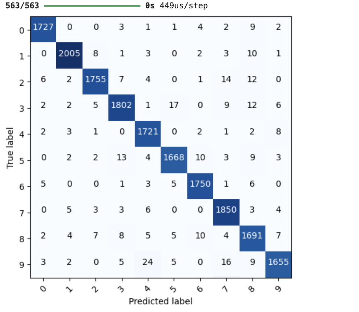
모델 예측 결과 - confusion matrix

우리가 만든 Keras 모델의 예측 결과를 실제 정답과 비교해 confusion matrix로도 보여줄 수 있다.

import itertools
from sklearn.metrics import confusion_matrix

def plot_confusion_matrix(model_input, feature, label, class_info):
	#예측값 얻음
    pred = model_input.predict(feature)
    #confusion matrix 계산
    cnf_matrix = confusion_matrix(np.argmax(label, axis=1), np.argmax(pred, axis=1))

    plt.figure()
    #matplotlib로 시각화
    plt.imshow(cnf_matrix, interpolation='nearest', cmap=plt.cm.Blues)
    tick_marks = np.arange(len(class_info))
    # confusion matrix 축에 숫자 표시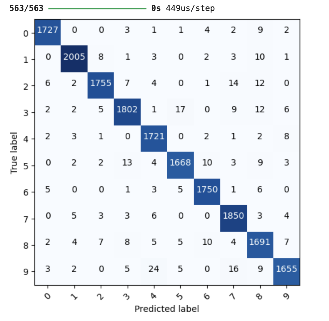![](https://velog.velcdn.com/images/onegyeol/post/fdd7ce5e-656e-4315-80d2-f9dd26d7f602/image.png)

    plt.xticks(tick_marks, class_info, rotation=45)
    plt.yticks(tick_marks, class_info)

    thresh = cnf_matrix.max() / 2.0
    
    # 각 셀 안에 숫자 출력, 값이 큰 경우는 하얀색으로 표시
    for i, j in itertools.product(range(cnf_matrix.shape[0]), range(cnf_matrix.shape[1])):
        plt.text(j, i, str(cnf_matrix[i, j]), horizontalalignment="center",\
                 color="white" if cnf_matrix[i, j] > thresh else "black")

	# 레이블 정리
    plt.tight_layout()
    plt.ylabel('True label')
    plt.xlabel('Predicted label')
    plt.show()

labels = ['0','1','2','3','4','5','6','7','8','9']
plot_confusion_matrix(mlp_model, X_test, Y_test, class_info=labels)

전체 코드

import numpy as np
import pandas as pd
import matplotlib.pyplot as plt
from sklearn.model_selection import train_test_split
from sklearn.metrics import confusion_matrix
from tensorflow.keras import utils
from tensorflow.keras.models import Model, Sequential
from tensorflow.keras.layers import Input, Dense, Conv2D, MaxPool2D, UpSampling2D, Flatten, Reshape, Embedding, LSTM
from tensorflow.keras.callbacks import EarlyStopping
from tensorflow.keras.preprocessing.text import Tokenizer
from tensorflow.keras.preprocessing.sequence import pad_sequences
from tensorflow.keras.optimizers import SGD

mnist_csv = pd.read_csv('./mnist_train.csv', header=None, skiprows=1).values
train, test = train_test_split(mnist_csv, test_size=0.3, random_state=1)

#train의 전체 행 저장+Y만 출력, 앞에 빼고 출력(X train)
Y_train, X_train = utils.to_categorical(train[:,0]), train[:,1:]

#test의 전체 행 중 Y만 출력, 앞에 Y빼고 저장
Y_test, X_test = utils.to_categorical(test[:,0]), test[:,1:]

#정규화
X_train = X_train / 255.0
X_test = X_test / 255.0

mlp_model = Sequential()
mlp_model.add(Dense(512, activation='sigmoid', input_shape=(784,))) # 입력층
mlp_model.add(Dense(256, activation='sigmoid'))
mlp_model.add(Dense(10, activation='softmax')) # 출력층 (0~9)
mlp_model.summary()

mlp_model.compile(loss='categorical_crossentropy', optimizer='adam', metrics=['accuracy'])

model_history = mlp_model.fit(X_train, Y_train, validation_data=(X_test, Y_test),\
                            epochs=15, batch_size=512, shuffle=True, verbose=2)