🎄 결정 트리

- 분류와 회귀 문제에 널리 사용하는 모델

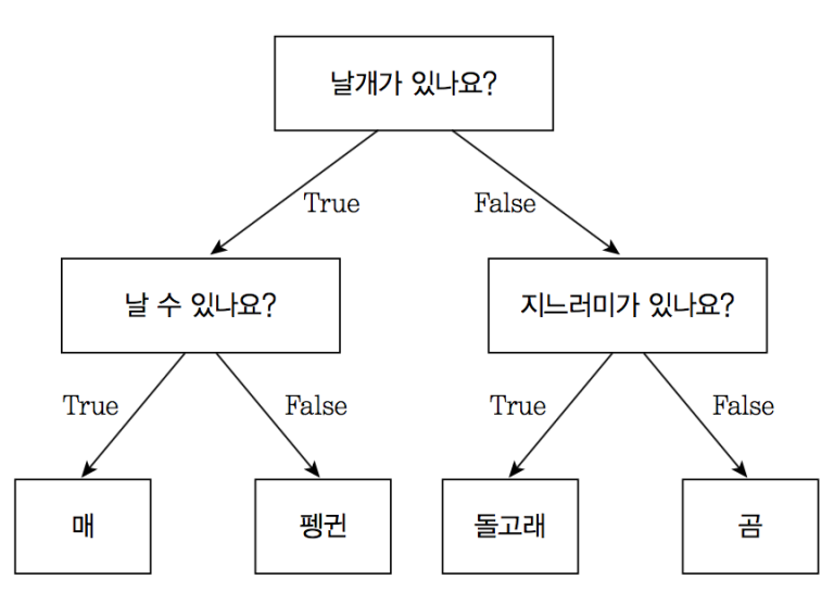
• 기본적으로 결정에 다다르기 위해 예/아니오 질문을 이어나가면서 학습
• 맨 위 노드 : 루트노드
• 트리노드는 질문이나 정답을 담은 네모상자
• 엣지는 질문의 답과 다음 질문을 연결
• 마지막 노드 : 리프(leaf)라고 함
• 모델을 직접 만드는 대신 지도 학습 방식으로 데이터로부터 학습

---

👩‍⚕️ DecisionTreeClassifier 사용하여 유방암 양성(2), 악성(4)

🐼 준비

from sklearn import preprocessing
from sklearn.model_selection import train_test_split
from sklearn import tree
from sklearn import metrics

import pandas as pd
import numpy as np

# 한글 깨짐 방지
import matplotlib as mpl
import matplotlib.pyplot as plt

%config InlineBackend.figure_format = 'retina'

!apt -qq -y install fonts-nanum

import matplotlib.font_manager as fm
fontpath = '/usr/share/fonts/truetype/nanum/NanumBarunGothic.ttf'
font = fm.FontProperties(fname=fontpath, size=9)
plt.rc('font', family='NanumBarunGothic') 
mpl.font_manager._rebuild()

데이터 준비하고 확인

# UCI ML Repository 제공하는 Breast Cancer 데이터셋 가져오기
uci_path = 'https://archive.ics.uci.edu/ml/machine-learning-databases/\breast-cancer-wisconsin/breast-cancer-wisconsin.data'
df = pd.read_csv(uci_path, header=None)

# 열 이름 지정
df.columns = ['id', 'clump', 'cell_size', 'cell_shape', 'adhesion', 'epithlial', 'bare_nuclei', 'chromatin', 'normal_nucleoli', 'mitoses', 'class']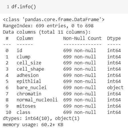

• 

👀 bare_nuclei만 object인 것에 의문 -> unique()로 확인

df['bare_nuclei'].unique()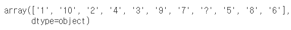

• 

👀 '?' 때문임을 알 수 있음 -> '?' 를 없애기 위해서 다음의 과정을 따름

1) '?' -> np.nan으로 변경하고 수를 확인

df['bare_nuclei'].replace('?', np.nan, inplace=True)
df['bare_nuclei'].isna().sum() # 16개의 물음표를 np.nan변환

2) NaN 데이터 삭제

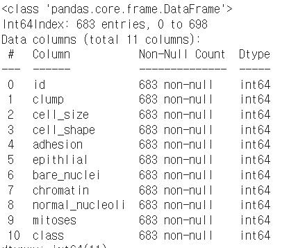
df.dropna(subset=['bare_nuclei'], axis=0, inplace=True)

3) bare_nuclei 컬럼 형변환 int

df['bare_nuclei'] = df['bare_nuclei'].astype('int')

df.info() 결과 type이 int로 변환되었음

---

데이터 분리하기

X = df[['clump', 'cell_size', 'cell_shape', 'adhesion', 'epithlial',
              'bare_nuclei', 'chromatin', 'normal_nucleoli', 'mitoses']]
y = df['class']

# X 독립변수 데이터를 정규화
X = preprocessing.StandardScaler().fit(X).transform(X)
X

# train, test set 분리(7:3)
X_train, X_test, y_train, y_test = train_test_split(X, y, test_size=0.3, random_state=7)
print('X_train.shape : ', X_train.shape)
print('X_test.shape : ', X_test.shape)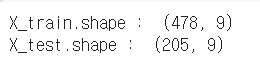

• 

---

DecisionTree 분류모델 설정

# 모델 객체 생성 (최적의 속성을 찾기 위해 criterion='entropy'적용) * 적정한 레벨 값 찾는 것이 중요
tree_model = tree.DecisionTreeClassifier(criterion='entropy', max_depth = 5) # 5개로만 모델 구성

모델 학습, 예측

# 모델 학습
tree_model.fit(X_train, y_train)
# 모델 예측
y_pred = tree_model.predict(X_test)

모델 성능평가

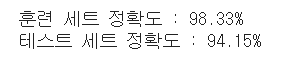
print('훈련 세트 정확도 : {:.2f}%'.format(tree_model.score(X_train, y_train)*100))
print('테스트 세트 정확도 : {:.2f}%'.format(tree_model.score(X_test, y_test)*100))

• 

tree_report = metrics.classification_report(y_test, y_pred)
print(tree_report)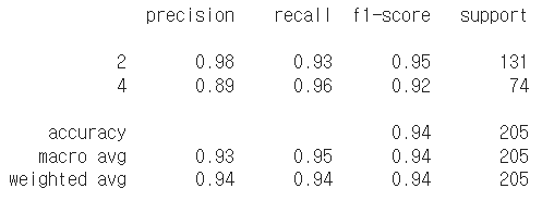

---

결정트리 그래프그리기

from sklearn.tree import export_graphviz
export_graphviz(tree_model, out_file='tree.dot', class_names=['악성','양성'],
                feature_names=df.columns[1:10], impurity=False, filled=True)

import graphviz
with open('tree.dot') as f:
  dot_graph = f.read()
display(graphviz.Source(dot_graph))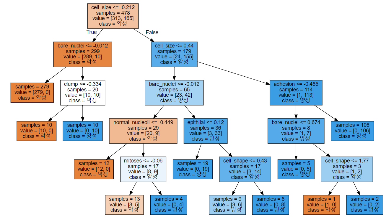

---

🎄 결정트리 앙상블

• 랜덤 포레스트 구축
  회귀와 분류에 있어서 가장 널리 사용되는 머신러닝 알고리즘
  텍스트 데이터같이 매우 차원이 높고 희소한 데이터들에는 잘 작동하지 않음

• 그래디언트 부스팅 회귀트리
  여러개의 결정 트리를 묶어 강력한 모델을 만듦

---

🧑‍⚕️ Ensemble Modeling Heart Disease 분류모델 비교

🐼 준비

데이터 다운로드 : https://archive.ics.uci.edu/ml/datasets/heart+disease

# 라이브러리 임포트
import numpy as np
import pandas as pd

import matplotlib.pyplot as plt
import seaborn as sns
import plotly.express as px

from sklearn.model_selection import train_test_split
from sklearn.preprocessing import StandardScaler

from sklearn.linear_model import LogisticRegression
from sklearn.tree import DecisionTreeClassifier
from sklearn.ensemble import RandomForestClassifier
from sklearn.ensemble import GradientBoostingClassifier

from sklearn import metrics

# 데이터 준비
df = pd.read_csv('/content/heart.csv')

데이터 전처리

카테고리(범주형) 컬럼 -> Dtype category -> 원핫인코딩
숫자형(연속형) 컬럼 -> 정규화

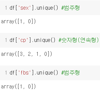
• 컬럼들 unique()로 확인해보기
  

# 범주형
categorical_var = ['sex', 'cp', 'fbs', 'restecg', 'exng', 'slp', 'caa', 'thall']
df[categorical_var] = df[categorical_var].astype('category')
df.info()

# 숫자형
numberic_var = [i for i in df.columns if i not in categorical_var][:-1] # categorical_var이 아닌 컬럼들

---

데이터분석

sns.countplot(df.sex) # sex (1 = male; 0 = female)

👀 남성(1)의 비율이 높음

---

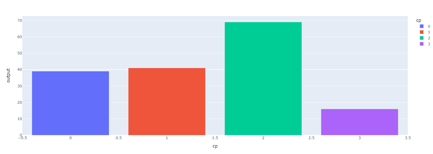
px.bar(df.groupby('cp').sum().reset_index()[['cp', 'output']], x='cp', y='output',color='cp')

cp : chest pain type

-- Value 1: typical angina
-- Value 2: atypical angina
-- Value 3: non-anginal pain
-- Value 4: asymptomatic

---

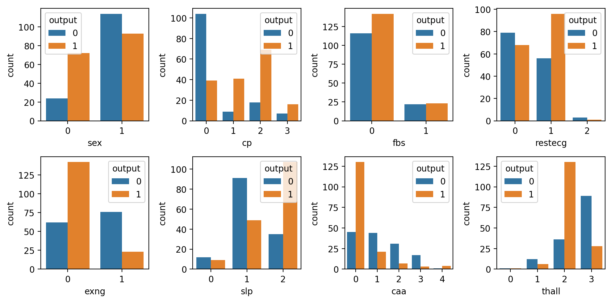
범주형 변수(categorical_var)와 output(y) 관계 시각화

fig, ax = plt.subplots(2,4, figsize=(10,5), dpi=200)
for axis, cat_var in zip(ax.ravel(), categorical_var):
  sns.countplot(x=cat_var, data=df, hue='output', ax=axis)
plt.tight_layout()

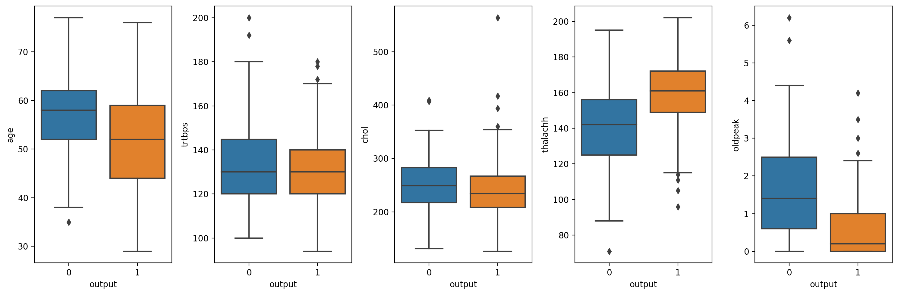
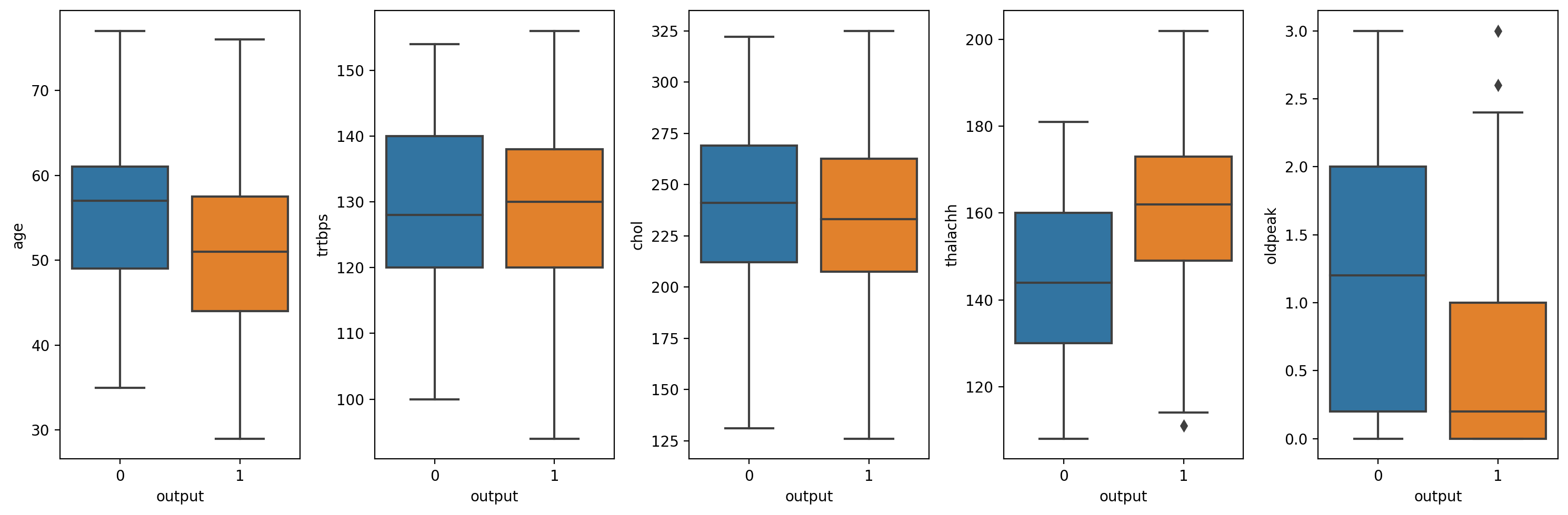
수치형(numberic_var)와 output(y)관계 시각화

fig, ax = plt.subplots(1, 5, figsize=(15,5), dpi=200)
for axis, num_var in zip(ax.ravel(), numberic_var):
  sns.boxplot(y=num_var, data=df, x='output', ax=axis)
plt.tight_layout()

수치형(numberic_var) 컬럼 중 나이 컬럼을 제거하고 5%의 이상치를 제거

trtbps , chol, oldpeak : 상위 5% 이상치 제거
thalachh : 하위 5% 이상치 제거

df = df[df['trtbps'] < df['trtbps'].quantile(0.95)] # 100% - 5% = 95%만
df = df[df['chol'] < df['chol'].quantile(0.95)]
df = df[df['oldpeak'] < df['oldpeak'].quantile(0.95)]
df = df[df['thalachh'] > df['thalachh'].quantile(0.05)]

수치형(numberic_var)와 output(y)관계 시각화

# subplot은 두개의 값을 return 하기 때문에 변수 두개 필요
fig, ax = plt.subplots(1, 5, figsize=(15,5), dpi=200)
for axis, num_var in zip(ax.ravel(), numberic_var):
  sns.boxplot(y=num_var, data=df, x='output', ax=axis)
plt.tight_layout()

---

데이터 분리하기

X = df.iloc[:, :-1] # iloc[row,column]
y = df['output']

# 범주형 -> 원핫인코딩
temp_x = pd.get_dummies(X[categorical_var])

# 원핫인코딩 컬럼 추가
X_modified = pd.concat([X, temp_x], axis=1)

# 기존 컬럼 삭제
X_modified.drop(categorical_var, axis=1, inplace=True)
X_modified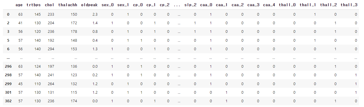

# 수치형 변수 -> 정규화 -> 스케일링
X_modified[numberic_var] = StandardScaler().fit_transform(X_modified[numberic_var])
X_modified.head()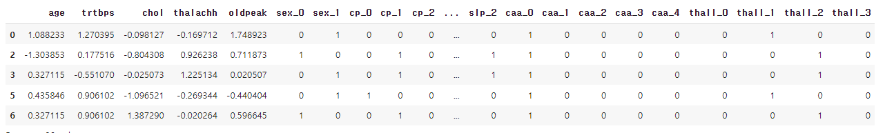

# test, train 데이터 분리
# 80:20 비율로 분리
X_train, X_test, y_train, y_test = train_test_split(X_modified, y, test_size=0.2, random_state=7)

---

머신러닝 모델 설정 및 학습

1) LogisticRegression

logreg = LogisticRegression(C=0.301).fit(X_train, y_train)
print('logreg 훈련 세트 정확도 : {:.5f}%'.format(logreg.score(X_train, y_train)*100))
print('logreg 테스트 세트 정확도 : {:.5f}%'.format(logreg.score(X_test, y_test)*100)) 

logreg 훈련 세트 정확도 : 88.82979%
logreg 테스트 세트 정확도 : 85.41667%

2) DecisionTree

tree = DecisionTreeClassifier(max_depth=5, min_samples_leaf=10, min_samples_split=40).fit(X_train, y_train)
print('DecisionTree 훈련 세트 정확도 : {:.5f}%'.format(tree.score(X_train, y_train)*100))
print('DecisionTree 테스트 세트 정확도 : {:.5f}%'.format(tree.score(X_test, y_test)*100)) 

DecisionTree 훈련 세트 정확도 : 81.91489%
DecisionTree 테스트 세트 정확도 : 81.25000%

3) RandomForest

random = RandomForestClassifier(n_estimators=400, random_state=7).fit(X_train, y_train)
print('RandomForest 훈련 세트 정확도 : {:.5f}%'.format(random.score(X_train, y_train)*100))
print('RandomForest 테스트 세트 정확도 : {:.5f}%'.format(random.score(X_test, y_test)*100)) 

RandomForest 훈련 세트 정확도 : 100.00000%
RandomForest 테스트 세트 정확도 : 83.33333%

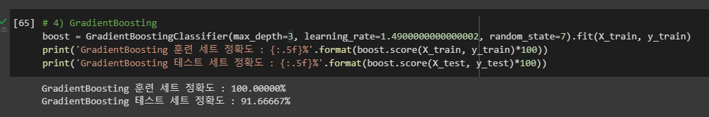
4) GradientBoosting

boost = GradientBoostingClassifier(max_depth=2, learning_rate=0.05).fit(X_train, y_train)
print('GradientBoosting 훈련 세트 정확도 : {:.5f}%'.format(boost.score(X_train, y_train)*100))
print('GradientBoosting 테스트 세트 정확도 : {:.5f}%'.format(boost.score(X_test, y_test)*100)) 

GradientBoosting 훈련 세트 정확도 : 93.61702%
GradientBoosting 테스트 세트 정확도 : 85.41667%

👀 여러 요인들(max_depth, n_estimators)을 바꾸면 정확도가 달라질 수 있음!

---

테스트 세트 정확도 높이기 !

🐼 우리조 🥰 3조(1등) 🥰

---

📰 지도학습 알고리즘 요약 정리

각 데이터 모델의 특징

• 최근접이웃 : 작은 데이터셋일 경우, 기본 모델로서 좋고 설명하기 쉬움
• 선형 모델 : 첫번째로 시도할 알고리즘, 대용량 데이터셋 가능, 고차원 데이터에 가능
• 나이브 베이즈 : 분류만 가능, 선형 모델보다 훨씬 빠름, 대용량 데이터셋과 고차원 데이터에 가능, 선형 모델보다 덜 정확함
• 결정 트리 : 매우 빠름, 데이터 스케일 조정이 필요 없음, 시각화하기 좋고 설명하기 쉬움
• 랜덤 포레스트 : 결정트리 하나보다 거의 항상 좋은 성능을 냄, 매우 안정적이고 강력, 데이터 스케일 조정 필요없음, 고차원 희소 데이터에는 안맞음
• 그래디언트 부스트 결정 트리 : 랜덤 포레스트보다 조금 더 성능이 좋음, 랜덤 포레스트보다 학습은 느리나 예측은 빠르고 메모리를 조금 사용, 랜덤 포레스트보다 매개변수 튜닝 많이 필요
• SVM : 비슷한 의미의 특성으로 이뤄진 중간 규모 데이터셋에 잘 맞음, 데이터 스케일 조정 필요, 매개변수에 민감
• 신경망 : 특별히 대용량 데이터셋에서 매우 복잡한 모델을 만들 수 있음, 선택과 데이터스케일에 민감, 큰 모델은 학습이 오래걸림