ᄂ 😄 [8 일차] : EXPLORATION 02. Iris 품종 분류

백건·2022년 1월 21일

AIFFEL AIFFEL WEEK02 EXPLORATION 아이펠

[AIFFEL] 아이펠 인공지능 전문가 과정

목록 보기

9/32

Iris의 세 가지 품종, 분류해볼 수 있겠어요?

들어가며

학습 목표

scikit-learn에 내장된 예제 데이터셋의 종류를 알고 활용할 수 있다.
scikit-learn에 내장된 분류 모델들을 학습시키고 예측해 볼 수 있다.
모델의 성능을 평가하는 지표의 종류에 대해 이해하고, 활용 및 확인해 볼 수 있다.
Decision Tree, XGBoost, RandomForest, 로지스틱 회귀 모델을 활용해서 간단하게 학습 및 예측해 볼 수 있다.
데이터셋을 사용해서 스스로 분류 기초 실습을 진행할 수 있다.

학습 전제

scikit-learn을 활용해서 머신러닝을 시도해본 적이 없다.
scikit-learn에 내장된 분류 모델을 활용해본 적이 없다.
지도학습의 분류 실습을 해 본 적이 없다.
머신러닝 모델을 학습시켜보고, 그 성능을 평가해본 적이 없다.

Iris의 세 가지 품종, 분류해 볼까요?

붓꽃 분류 문제

pip install scikit-learn
pip install matplotlib

분류하기 위한 데이터

사이킷런(scikit-learn)에 내장된 데이터 사용
붓꽃 데이터가 내장되어 있음.(그래서 쓴다고..ㅋ)

사이킷런(scikit-learn)

Toy datasets : 7가지 , 간단하고 작은 데이터셋
- boston
- iris
- diabetes
- digits
- linnerrud
- wine
- breast
- cancer

Real world datasets : 7가지 , 복잡하고 현실 세계 반영한 데이터셋
- olivetti faces
- 20 newsgroups
- labeled faces
- forest covertype
- RCV1
- Kddcup 99
- California housin

petal은 꽃잎, sepal은 꽃받침

시작전 데이터를 정확히 자세 확인

Total data : 150(Instance)
Attributes : 4
- sepal
  - length
  - width
- petal
  - length
  - width
Class
- Iris
  - Setosa
  - Versicolour
  - virginica

데이터 준비, 그리고 자세히 살펴보기는 기본!

데이터 확인.

#  sklearn 라이브러리의 datasets 패키지 안 load_iris를 import 
#  iris 데이터를 로딩

from sklearn.datasets import load_iris

iris = load_iris()

print(dir(iris)) # iris 객체가 어떤 변수와 메서드를 가지고 있나
# dir()는 객체가 어떤 변수와 메서드를 가지고 있는지 나열함

['DESCR', 'data', 'data_module', 'feature_names', 'filename', 'frame', 'target', 'target_names']

담긴 정보 확인

#  iris에는 어떤 정보들이 담겼을지, keys() 라는 메서드로 확인
iris.keys()

dict_keys(['data', 'target', 'frame', 'target_names', 'DESCR', 'feature_names', 'filename', 'data_module'])

7가지 : 'data', 'target', 'frame', 'target_names', 'DESCR', 'feature_names', 'filename'

->>data_module 은???

중요 데이터 변수에 저장

#  중요한 데이터는 iris_data 변수에 저장

iris_data = iris.data

데이터 크기 확인.

print(iris_data.shape) 
#shape는 배열의 형상정보를 출력

(150, 4)

150개 데이터

4종류의 정보

샘플데이터 확인.

iris_data[0] # 0번 index에 접근接近

array([5.1, 3.5, 1.4, 0.2])

해결할 문제 확인. -> 라벨 or 타겟

붓꽃의 꽃잎 길이와 폭 / 꽃받침 길이와 폭 이용

붓꽃의 종류가 setosa, versicolor, virginica 세 가지 중 무엇인지.

타겟 정보 확인

iris_label = iris.target  # iris_label 변수에 타겟정보 저장
print(iris_label.shape)   # 변수 크기 출력
iris_label                #

(150,)





array([0, 0, 0, 0, 0, 0, 0, 0, 0, 0, 0, 0, 0, 0, 0, 0, 0, 0, 0, 0, 0, 0,
       0, 0, 0, 0, 0, 0, 0, 0, 0, 0, 0, 0, 0, 0, 0, 0, 0, 0, 0, 0, 0, 0,
       0, 0, 0, 0, 0, 0, 1, 1, 1, 1, 1, 1, 1, 1, 1, 1, 1, 1, 1, 1, 1, 1,
       1, 1, 1, 1, 1, 1, 1, 1, 1, 1, 1, 1, 1, 1, 1, 1, 1, 1, 1, 1, 1, 1,
       1, 1, 1, 1, 1, 1, 1, 1, 1, 1, 1, 1, 2, 2, 2, 2, 2, 2, 2, 2, 2, 2,
       2, 2, 2, 2, 2, 2, 2, 2, 2, 2, 2, 2, 2, 2, 2, 2, 2, 2, 2, 2, 2, 2,
       2, 2, 2, 2, 2, 2, 2, 2, 2, 2, 2, 2, 2, 2, 2, 2, 2, 2])

# 라벨의 이름은 target_names에서 확인
iris.target_names

array(['setosa', 'versicolor', 'virginica'], dtype='<U10')

0 이라면 setosa,

1 이라면 versicolor,

2 라면 virginica

print(iris.DESCR) # DESCR에는 데이터셋의 설명

.. _iris_dataset:

Iris plants dataset
--------------------

**Data Set Characteristics:**

    :Number of Instances: 150 (50 in each of three classes)
    :Number of Attributes: 4 numeric, predictive attributes and the class
    :Attribute Information:
        - sepal length in cm
        - sepal width in cm
        - petal length in cm
        - petal width in cm
        - class:
                - Iris-Setosa
                - Iris-Versicolour
                - Iris-Virginica
                
    :Summary Statistics:

    ============== ==== ==== ======= ===== ====================
                    Min  Max   Mean    SD   Class Correlation
    ============== ==== ==== ======= ===== ====================
    sepal length:   4.3  7.9   5.84   0.83    0.7826
    sepal width:    2.0  4.4   3.05   0.43   -0.4194
    petal length:   1.0  6.9   3.76   1.76    0.9490  (high!)
    petal width:    0.1  2.5   1.20   0.76    0.9565  (high!)
    ============== ==== ==== ======= ===== ====================

    :Missing Attribute Values: None
    :Class Distribution: 33.3% for each of 3 classes.
    :Creator: R.A. Fisher
    :Donor: Michael Marshall (MARSHALL%PLU@io.arc.nasa.gov)
    :Date: July, 1988

The famous Iris database, first used by Sir R.A. Fisher. The dataset is taken
from Fisher's paper. Note that it's the same as in R, but not as in the UCI
Machine Learning Repository, which has two wrong data points.

This is perhaps the best known database to be found in the
pattern recognition literature.  Fisher's paper is a classic in the field and
is referenced frequently to this day.  (See Duda & Hart, for example.)  The
data set contains 3 classes of 50 instances each, where each class refers to a
type of iris plant.  One class is linearly separable from the other 2; the
latter are NOT linearly separable from each other.

.. topic:: References

   - Fisher, R.A. "The use of multiple measurements in taxonomic problems"
     Annual Eugenics, 7, Part II, 179-188 (1936); also in "Contributions to
     Mathematical Statistics" (John Wiley, NY, 1950).
   - Duda, R.O., & Hart, P.E. (1973) Pattern Classification and Scene Analysis.
     (Q327.D83) John Wiley & Sons.  ISBN 0-471-22361-1.  See page 218.
   - Dasarathy, B.V. (1980) "Nosing Around the Neighborhood: A New System
     Structure and Classification Rule for Recognition in Partially Exposed
     Environments".  IEEE Transactions on Pattern Analysis and Machine
     Intelligence, Vol. PAMI-2, No. 1, 67-71.
   - Gates, G.W. (1972) "The Reduced Nearest Neighbor Rule".  IEEE Transactions
     on Information Theory, May 1972, 431-433.
   - See also: 1988 MLC Proceedings, 54-64.  Cheeseman et al"s AUTOCLASS II
     conceptual clustering system finds 3 classes in the data.
   - Many, many more ...

# feature_names에는 다음과 같이 4개의 각 feature에 대한 설명
iris.feature_names

['sepal length (cm)',
 'sepal width (cm)',
 'petal length (cm)',
 'petal width (cm)']

# filename에는 데이터셋의 전체 이름
iris.filename

'iris.csv'

csv 파일이군...

첫 번째 머신러닝 실습, 간단하고도 빠르게!

머신러닝 모델을 학습시키기 위한 문제지와 정답지 준비

pandas = pd = 판다스

라이브러리

파이썬에서 표 형태로 이루어진 2차원 배열 데이터를 다루는 데에 가장 많이 쓰이는 도구

표 데이터를 활용해서 데이터 분석

대형 데이터의 여러 통계량을 다루는 것에 최적화

import pandas as pd

print(pd.__version__)

1.3.5

# 붓꽃 데이터셋을 pandas가 제공하는 DataFrame 이라는 자료형으로 변환
iris_df = pd.DataFrame(data=iris_data, columns=iris.feature_names)
# iris_df

# DataFrame 을 만들면서 data에는 iris_data를 넣어주고, 각 컬럼에는 feature_names로 이름을 붙여줌

# label 컬럼 추가
iris_df["label"] = iris.target
iris_df

	sepal length (cm)	sepal width (cm)	petal length (cm)	petal width (cm)	label
0	5.1	3.5	1.4	0.2	0
1	4.9	3.0	1.4	0.2	0
2	4.7	3.2	1.3	0.2	0
3	4.6	3.1	1.5	0.2	0
4	5.0	3.6	1.4	0.2	0
...	...	...	...	...	...
145	6.7	3.0	5.2	2.3	2
146	6.3	2.5	5.0	1.9	2
147	6.5	3.0	5.2	2.0	2
148	6.2	3.4	5.4	2.3	2
149	5.9	3.0	5.1	1.8	2

150 rows × 5 columns

문제지와 정답지 준비

4가지의 feature 데이터들은 바로 머신러닝 모델이 풀어야 하는 문제지

-> [5.1, 3.5, 1.4, 0.2]라는 문제가 주어진다면 모델은 0, 즉 setosa라는 답을 맞혀야 하는 것

label 데이터는 머신러닝 모델에게 정답지

-> 0, 1, 2와 같이 표현된 label 데이터

문제지 :

머신러닝 모델에게 입력되는 데이터.

feature라고 부르기도 함.

변수 이름으로는 X를 많이 사용.

정답지 :

머신러닝 모델이 맞혀야 하는 데이터.

label 또는 target이라고 부름.

변수 이름으로는 y를 많이 사용

머신러닝 모델을 학습시키기 위한 장치

학습에 사용하는 training dataset과
모델의 성능을 평가하는 데 사용하는 test dataset으로 데이터셋을 나누는 작업
데이터셋을 분리하는 것은 scikit-learn이 제공하는 train_test_split 이라는 함수

- sklearn.model_selection 패키지의 train_test_split을 활용
- training dataset과 test dataset을 분리

from sklearn.model_selection import train_test_split

X_train, X_test, y_train, y_test = train_test_split(iris_data,      
                                                    # iris_data는 문제지 :  feature
                                                    iris_label,     
                                                    # 맞춰야 할 정답값 : Label(3가지중)
                                                    test_size=0.2,  
                                                    # test dataset의 크기를 조절 : 전체의 20%만 테스트데이터로 사용
                                                    random_state=7) 
                                                    # train 데이터와 test 데이터를 분리(split)하는데 적용되는 랜덤성

print('X_train 개수: ', len(X_train),', X_test 개수: ', len(X_test))

X_train 개수:  120 , X_test 개수:  30

# X_train부터 y_test까지 만들어진 데이터셋을 확인
X_train.shape, y_train.shape

((120, 4), (120,))

X_test.shape, y_test.shape

((30, 4), (30,))

20%의 데이터는 test 데이터셋

나머지 80%의 데이터는 train 데이터셋

y_train, y_test

(array([2, 1, 0, 2, 1, 0, 0, 0, 0, 2, 2, 1, 2, 2, 1, 0, 1, 1, 2, 0, 0, 0,
        2, 0, 2, 1, 1, 1, 0, 0, 0, 1, 2, 1, 1, 0, 2, 0, 0, 2, 2, 0, 2, 0,
        1, 2, 1, 0, 1, 0, 2, 2, 1, 0, 0, 1, 2, 0, 2, 2, 1, 0, 1, 0, 2, 2,
        0, 0, 2, 1, 2, 2, 1, 0, 0, 2, 0, 0, 1, 2, 2, 1, 1, 0, 2, 0, 0, 1,
        1, 2, 0, 1, 1, 2, 2, 1, 2, 0, 1, 1, 0, 0, 0, 1, 1, 0, 2, 2, 1, 2,
        0, 2, 1, 1, 0, 2, 1, 2, 1, 0]),
 array([2, 1, 0, 1, 2, 0, 1, 1, 0, 1, 1, 1, 0, 2, 0, 1, 2, 2, 0, 0, 1, 2,
        1, 2, 2, 2, 1, 1, 2, 2]))

첫 번째 머신러닝 모델 학습시키기

머신러닝

지도학습(Supervised Learning)
- 지도받을 수 있는, 즉 정답이 있는 문제에 대해 학습하는 것
  - 분류(Classification)
    - 입력받은 데이터를 특정 카테고리 중 하나로 분류해내는 문제
  - 회귀(Regression)
    - 입력받은 데이터에 따라 특정 필드의 수치를 맞히는 문제

비지도학습(Unsupervised Learning)
- 비지도 학습은 정답이 없는 문제를 학습하는 것

붓꽃은
Supervised Learning / Classification

분류모델

Decision Tree Model

참고 의사결정나무
의사 결정을 할, 즉 데이터를 분리할 어떤 경계를 찾아내어 데이터를 체에 거르듯 한 단계씩 분류해나가는 모델
데이터를 분리해나가는 모습이 나무를 뒤집어 놓은 것과 같은 모양
순도(homogeneity)가 증가
불순도(impurity) 혹은 불확실성(uncertainty)이 최대한 감소하도록 하는 방향으로 학습을 진행
- 순도가 증가/불확실성이 감소하는 걸 두고 정보이론에서는 정보획득(information gain)
- 데이터가 균일한 정도를 나타내는 지표, 즉 순도
- 순도를 계산하는 3가지 방식
  - 엔트로피(entropy)
  - 지니계수(Gini Index)
  - 오분류오차(misclassification error)
    - 오분류오차는 엔트로피나 지니계수와 더불어 불순도를 측정할 수 있음
    - 나머지 두 지표와 달리 미분이 불가능한 점 때문에 자주 쓰이지는 않음
학습과정
- 입력 변수 영역을 두 개로 구분하는 재귀적 분기(recursive partitioning) 과정
- 자세하게 구분된 영역을 통합하는 가지치기(pruning) 과정
  - 모든 terminal node의 순도가 100%인 상태를 Full tree
  - Full tree를 생성한 뒤 적절한 수준에서 terminal node를 결합해주어야 함
    - 분기가 너무 많아서 학습데이터에 과적합(overfitting)할 염려
    - 처음에는 새로운 데이터에 대한 오분류율이 감소
    - 일정 수준 이상이 되면 오분류율이 되레 증가하는 현상이 발생
    - 분기를 합치는(merge) 개념
  - 비용함수(cost function)
    - 𝐶𝐶(𝑇)=𝐸𝑟𝑟(𝑇)+𝛼×𝐿(𝑇)
      - CC(T)=의사결정나무의 비용 복잡도
        (=오류가 적으면서 terminal node 수가 적은 단순한 모델일 수록 작은 값)
      - ERR(T)=검증데이터에 대한 오분류율
      - L(T)=terminal node의 수 (구조의 복잡도)
      - Alpha=ERR(T)와 L(T)를 결합하는 가중치
        (사용자에 의해 부여됨, 보통 0.01~0.1의 값을 씀)
장점
- 계산복잡성 대비 높은 예측 성능을 내는 것
- 변수 단위로 설명력을 지닌다는 강점
단점
- 결정경계(decision boundary)가 데이터 축에 수직이어서 특정 데이터에만 잘 작동할 가능성
대안
- RandomForest
  - 같은 데이터에 대해 의사결정나무를 여러 개 만들어 그 결과를 종합해 예측 성능을 높이는 기법

Decidion Tree 모델 사용법

# Decision Tree는 sklearn.tree 패키지 안에 DecisionTreeClassifier 라는 이름으로 내장

from sklearn.tree import DecisionTreeClassifier

# 모델을 import해서 가져오고, decision_tree 라는 변수에 모델을 저장

decision_tree = DecisionTreeClassifier(random_state=32)
print(decision_tree._estimator_type)

classifier

위 결과의 의미는?

모델 학습은 우리가 준비해 둔 X_train 와 y_train 데이터로
다음 한 줄이면 완료

decision_tree.fit(X_train, y_train) 
#모델 학습을 시키기 위해 준비해둔 X_train y_train로 의사결정 나무에 fit

DecisionTreeClassifier(random_state=32)

XGBoost

같은 데이터에 의사결정나무 여러 개를 동시에 적용해서 학습성능을 높이는 앙상블 기법
작동 방식
- 동일한 데이터로부터 복원추출을 통해
- 30개 이상의 데이터 셋을 만들어
- 각각에 의사결정나무를 적용한 뒤
- 학습 결과를 취합하는 방식
성능 지표는 단순정확도(accuracy)

RandomForest

로지스틱 회귀 모델

첫 번째 머신러닝 모델 평가하기

test 데이터로 예측

y_pred = decision_tree.predict(X_test)
y_pred

array([2, 1, 0, 1, 2, 0, 1, 1, 0, 1, 2, 1, 0, 2, 0, 2, 2, 2, 0, 0, 1, 2,
       1, 1, 2, 2, 1, 1, 2, 2])

X_test 데이터에는 정답인 label이 없고 feature 데이터만 존재

학습이 완료된 decision_tree 모델에

X_test 데이터로 predict를 실행하면

모델이 예측한 y_pred을 얻게 됨

모델은 총 30개의 데이터에 대해
array([2, 1, 0, 1, 2, 0, 1, 1, 0, 1, 2, 1, 0, 2, 0, 2, 2, 2, 0, 0, 1, 2,
1, 1, 2, 2, 1, 1, 2, 2])라는 예측 결과

실제 정답인 y_test와 비교해서 얼마나 맞았는지 확인

y_test

array([2, 1, 0, 1, 2, 0, 1, 1, 0, 1, 1, 1, 0, 2, 0, 1, 2, 2, 0, 0, 1, 2,
       1, 2, 2, 2, 1, 1, 2, 2])

알아보기 힘듦 ㅜㅜ

쉽게 비교하는 방법은

scikit-learn에서 성능 평가에 대한 함수들이 모여있는 sklearn.metrics 패키지를 이용

# 성능을 평가하는 다양한 척도 중 정확도(Accuracy) 확인
from sklearn.metrics import accuracy_score

accuracy = accuracy_score(y_test, y_pred)
accuracy

0.9

0.9는 수치는 90% 정도의 정확도

[[[총정리]]]다른 모델도 해 보고 싶다면? 코드 한 줄만 바꾸면 돼!

# 앞 내용 정리

# (1) 필요한 모듈 import
from sklearn.datasets import load_iris
from sklearn.model_selection import train_test_split
from sklearn.tree import DecisionTreeClassifier
from sklearn.metrics import classification_report

# (2) 데이터 준비
iris = load_iris()
iris_data = iris.data
iris_label = iris.target

# (3) train, test 데이터 분리
X_train, X_test, y_train, y_test = train_test_split(iris_data, 
                                                    iris_label, 
                                                    test_size=0.2, 
                                                    random_state=7)

# (4) 모델 학습 및 예측 -> 모델을 바꾸고 싶을 때 변경하는 부분
decision_tree = DecisionTreeClassifier(random_state=32)
decision_tree.fit(X_train, y_train)
y_pred = decision_tree.predict(X_test)

print(classification_report(y_test, y_pred))

              precision    recall  f1-score   support

           0       1.00      1.00      1.00         7
           1       0.91      0.83      0.87        12
           2       0.83      0.91      0.87        11

    accuracy                           0.90        30
   macro avg       0.91      0.91      0.91        30
weighted avg       0.90      0.90      0.90        30

Random Forest

Random Forest는 상위 모델들이 예측하는 편향된 결과보다,
다양한 모델들의 결과를 반영함으로써 더 다양한 데이터에 대한 의사결정 가능
Decision Tree를 여러 개
Decision Tree의 단점을 극복한 모델
- 앙상블(Ensemble) 기법
- 단일 모델을 여러 개 사용하는 방법을 취함으로써
  모델 한 개만 사용할 때의 단점을 집단지성으로 극복하는 개념
Random Forest는 각각의 의사 결정 트리를 만드는데 있어 쓰이는 요소들
(흡연 여부, 나이, 등등)을 무작위적으로 선정
30개 중 무작위로 일부만 선택하여,
그 선택된 일부 중 가장 건강 위험도를 알맞게 예측하는
한 가지 요소가 의사 결정 트리의 한 단계
의사결정 과정
1. 건강의 위험도를 예측하기 위해서는 많은 요소를 고려
  성별, 키, 몸무게, 지역, 운동량, 흡연유무, 음주 여부,
  혈당, 근육량, 기초 대사량 등 수많은 요소가 필요
2. Feature가 30개라 했을 때 30개의 Feature를 기반으로
  하나의 결정 트리를 만든다면 트리의 가지가 많아질 것이고,
  이는 오버피팅의 결과를 야기
  3.30개의 Feature 중 랜덤으로 5개의 Feature만 선택해서 하나의 결정 트리 생성
3. 계속 반복하여 여러 개의 결정 트리 생성
4. 여러 결정 트리들이 내린 예측 값들 중 가장 많이 나온 값을 최종 예측값으로 지정
5. 이렇게 의견을 통합하거나 여러 가지 결과를 합치는 방식을 앙상블(Ensemble)이라고 함
6. 하나의 거대한 (깊이가 깊은) 결정 트리를 만드는 것이 아니라 여러 개의 작은 결정 트리를 만드는 것
7. 분류 : 여러 개의 작은 결정 트리가 예측한 값들 중 가장 많은 값, 회귀 : 평균

# Random Forest는 sklearn.ensemble 패키지 내
from sklearn.ensemble import RandomForestClassifier

X_train, X_test, y_train, y_test = train_test_split(iris_data, 
                                                    iris_label, 
                                                    test_size=0.2, 
                                                    random_state=21)

random_forest = RandomForestClassifier(random_state=32)
random_forest.fit(X_train, y_train)
y_pred = random_forest.predict(X_test)

print(classification_report(y_test, y_pred))

              precision    recall  f1-score   support

           0       1.00      1.00      1.00        11
           1       1.00      0.83      0.91        12
           2       0.78      1.00      0.88         7

    accuracy                           0.93        30
   macro avg       0.93      0.94      0.93        30
weighted avg       0.95      0.93      0.93        30

다른 scikit-learn 내장 분류 모델

Support Vector Machine (SVM)

Support Vector와 Hyperplane(초평면)을 이용하여 분류를 수행
대표적인 선형 분류 알고리즘

2 차원 공간에서, 즉 데이터에 2개의 클래스만 존재할 때,

Decision Boundary(결정 경계): 두 개의 클래스를 구분해 주는 선
Support Vector: Decision Boundary에 가까이 있는 데이터
Margin: Decision Boundary와 Support Vector 사이의 거리

Margin이 넓을수록 새로운 데이터를 잘 구분할 수 있다. (Margin 최대화 -> robustness 최대화)

Kernel Trick: 저차원의 공간을 고차원의 공간으로 매핑해주는 작업.
데이터의 분포가 Linearly separable 하지 않을 경우
데이터를 고차원으로 이동시켜 Linearly separable하도록 만든다.
cost: Decision Boundary와 Margin의 간격 결정.
cost가 높으면 Margin이 좁아지고 train error가 작아진다.
그러나 새로운 데이터에서는 분류를 잘 할 수 있다.
cost가 낮으면 Margin이 넓어지고, train error는 커진다.
γ: 한 train data당 영향을 미치는 범위 결정.
γ가 커지면 영향을 미치는 범위가 줄어들고,
Decision Boundary에 가까이 있는 데이터만이 선의 굴곡에 영향을 준다.
따라서 Decision Boundary는 구불구불하게 그어진다. (오버피팅 초래 가능)
작아지면 데이터가 영향을 미치는 범위가 커지고,
대부분의 데이터가 Decision Boundary에 영향을 준다.
따라서 Decision Boundary를 직선에 가까워진다.

SVM 모델 사용법

from sklearn import svm
svm_model = svm.SVC()

print(svm_model._estimator_type)

classifier

# 분꽃에 코드를 적용
svm_model.fit(X_train, y_train)
y_pred = svm_model.predict(X_test)

print(classification_report(y_test, y_pred))

# 아래는 decision_tree

# decision_tree = DecisionTreeClassifier(random_state=32)
# decision_tree.fit(X_train, y_train)
# y_pred = decision_tree.predict(X_test)

# print(classification_report(y_test, y_pred))

              precision    recall  f1-score   support

           0       1.00      1.00      1.00        11
           1       0.91      0.83      0.87        12
           2       0.75      0.86      0.80         7

    accuracy                           0.90        30
   macro avg       0.89      0.90      0.89        30
weighted avg       0.91      0.90      0.90        30

Stochastic Gradient Descent Classifier (SGDClassifier)

SGD (Stochastic Gradient Descent)
배치 크기가 1인 경사하강법 알고리즘
확률적 경사하강법은 데이터 세트에서
무작위로 균일하게 선택한 하나의 예를 의존하여
각 단계의 예측 경사를 계산

<최소값을 찾는 과정>

배치

경사하강법에서 배치는 단일 반복에서 기울기를 계산하는 데 사용하는 예(data)의 총 개수
Gradient Descent 에서의 배치는 전체 데이터 셋라고 가정

엄청난 데이터 셋

만약에 훨씬 적은 계산으로 적절한 기울기를 얻을 수 있다면?

확률적 경사하강법(SGD)은 이 아이디어를 더욱 확장한 것
반복당 하나의 예(배치 크기 1)만을 사용
- '확률적(Stochastic)'이라는 용어는 각 배치를 포함하는 하나의 예가 무작위로 선택된다는 것
단점
- 반복이 충분하면 SGD가 효과는 있지만 노이즈가 심함
  -확률적 경사하강법의 여러 변형 함수의 최저점에 가까운 점을
  찾을 가능성이 높지만 항상 보장되지는 않음
단점 극복
- 미니 배치 확률적 경사하강법(미니 배치 SGD)는
  전체 배치 반복과 SGD 의 절충안
  - 무작위로 선택한 10개에서 1,000개 사이의 예로 구성
  - 미니 배치 SGD는 SGD의 노이즈를 줄이면서도
  전체 배치보다는 더 효율적

SGD Classifier 모델 사용법

from sklearn.linear_model import SGDClassifier
sgd_model = SGDClassifier()

print(sgd_model._estimator_type)


# 참고 SVM 사용법
        from sklearn import svm
        svm_model = svm.SVC()

        print(svm_model._estimator_type)

# SVM 적용 예 
        svm_model.fit(X_train, y_train)
        y_pred = svm_model.predict(X_test)

        print(classification_report(y_test, y_pred))

        
# Tree 사용법
from sklearn.tree import DecisionTreeClassifier
decision_tree = DecisionTreeClassifier(random_state=32)

print(decision_tree._estimator_type)

#Tree 적용 예
decision_tree = DecisionTreeClassifier(random_state=32)
decision_tree.fit(X_train, y_train)
y_pred = decision_tree.predict(X_test)

print(classification_report(y_test, y_pred))

  File "/tmp/ipykernel_379/2372895087.py", line 8
    from sklearn import svm
    ^
IndentationError: unexpected indent

# 코드를 입력하세요 적용 예
sgd_model.fit(X_train, y_train)
y_pred = sgd_model.predict(X_test)

print(classification_report(y_test, y_pred))

              precision    recall  f1-score   support

           0       1.00      1.00      1.00        11
           1       1.00      0.92      0.96        12
           2       0.88      1.00      0.93         7

    accuracy                           0.97        30
   macro avg       0.96      0.97      0.96        30
weighted avg       0.97      0.97      0.97        30

# 적용예 답안
sgd_model.fit(X_train, y_train)
y_pred = sgd_model.predict(X_test)

print(classification_report(y_test, y_pred))

              precision    recall  f1-score   support

           0       1.00      1.00      1.00        11
           1       0.86      1.00      0.92        12
           2       1.00      0.71      0.83         7

    accuracy                           0.93        30
   macro avg       0.95      0.90      0.92        30
weighted avg       0.94      0.93      0.93        30

Logistic Regression

가장 널리 알려진 선형 분류 알고리즘.
소프트맥스(softmas) 함수를 사용한 다중 클래스 분류 알고리즘
다중 클래스 분류를 위한 로지스틱 회귀를 소프트맥스 회귀(Softmax Regression)
이름은 회귀지만, 실제로는 분류를 수행

소프트맥스 함수

클래스가 N개일 때, N차원의 벡터가 각 클래스가 정답일 확률을 표현하도록 정규화를 해주는 함수.
예시는 4차원의 벡터를 입력으로 받아 3개의 클래스를 예측하는 경우의 소프트맥스 회귀의 동작 과정
3개의 클래스 중 1개의 클래스를 예측해야 하므로 소프트맥스 회귀의 출력은 3차원의 벡터
각 벡터의 차원은 특정 클래스일 확률
오차와 실제값의 차이를 줄이는 과정에서 가중치와 편향이 학습

Logistic Regression 모델 사용법

from sklearn.linear_model import LogisticRegression
logistic_model = LogisticRegression()

print(logistic_model._estimator_type)

# 참고 SGD 사용법

                    from sklearn.linear_model import SGDClassifier
                    sgd_model = SGDClassifier()
    
                    print(sgd_model._estimator_type)
    
# SDG 적용 예

                    sgd_model.fit(X_train, y_train)
                    y_pred = sgd_model.predict(X_test)
            
                    print(classification_report(y_test, y_pred))


# 참고 SVM 사용법
        from sklearn import svm
        svm_model = svm.SVC()

        print(svm_model._estimator_type)

# SVM 적용 예 
        svm_model.fit(X_train, y_train)
        y_pred = svm_model.predict(X_test)

        print(classification_report(y_test, y_pred))

        
# Tree 사용법
                from sklearn.tree import DecisionTreeClassifier
                decision_tree = DecisionTreeClassifier(random_state=32)

                print(decision_tree._estimator_type)

#Tree 적용 예
                decision_tree = DecisionTreeClassifier(random_state=32)
                decision_tree.fit(X_train, y_train)
                y_pred = decision_tree.predict(X_test)

                print(classification_report(y_test, y_pred))

  File "<tokenize>", line 22
    from sklearn import svm
    ^
IndentationError: unindent does not match any outer indentation level

# 적용 예
# 코드를 입력하세요
logistic_model.fit(X_train, y_train)
y_pred = logistic_model.predict(X_test)

print(classification_report(y_test, y_pred))

              precision    recall  f1-score   support

           0       1.00      1.00      1.00        11
           1       1.00      0.83      0.91        12
           2       0.78      1.00      0.88         7

    accuracy                           0.93        30
   macro avg       0.93      0.94      0.93        30
weighted avg       0.95      0.93      0.93        30

내 모델은 얼마나 똑똑한가? 다양하게 평가해 보기

머신러닝에서는 성능을 정확히 평가하고 개선하는 것이 매우 중요
정확도라는 척도를 통해 모델의 성능을 확인
모델의 성능을 평가하는 데에는 정확도뿐만 아니라 다른 척도들이 존재

정확도에는 함정이 있다

함정의 사례

from sklearn.datasets import load_digits

digits = load_digits()
digits.keys()

dict_keys(['data', 'target', 'frame', 'feature_names', 'target_names', 'images', 'DESCR'])

digits 라는 변수에 손글씨 데이터를 저장했고, 그 안에는 iris 데이터와 똑같이 몇 가지의 정보

# 가장 중요한 data를 먼저 확인
digits_data = digits.data
digits_data.shape

(1797, 64)

데이터는 총 1,797개,
각 데이터는 64개의 숫자.

# 1,797개의 데이터 중 첫 번째 데이터를 샘플로 확인
digits_data[0]

array([ 0.,  0.,  5., 13.,  9.,  1.,  0.,  0.,  0.,  0., 13., 15., 10.,
       15.,  5.,  0.,  0.,  3., 15.,  2.,  0., 11.,  8.,  0.,  0.,  4.,
       12.,  0.,  0.,  8.,  8.,  0.,  0.,  5.,  8.,  0.,  0.,  9.,  8.,
        0.,  0.,  4., 11.,  0.,  1., 12.,  7.,  0.,  0.,  2., 14.,  5.,
       10., 12.,  0.,  0.,  0.,  0.,  6., 13., 10.,  0.,  0.,  0.])

예상대로 64개의 숫자로 이루어진 배열(array)이 출력

숫자는 어떤 의미가 있을까요?

손글씨 데이터는 이미지 데이터. -> 각 숫자는 픽셀값 의미
길이 64의 숫자 배열은 사실 (8 x 8) 크기의 이미지를 일렬로 쭉 펴놓은 것

이미지를 보기 위해서는 matplotlib이라는 라이브러리가 필요.

matplotlib.pyplot을 plt라는 이름으로 가져오고,
이미지를 현재 화면에 보여주기 위해
%matplotlib inline이라는 코드를 추가

# 일렬로 펴진 64개 데이터를 (8, 8)로 reshape

import matplotlib.pyplot as plt
%matplotlib inline

plt.imshow(digits.data[0].reshape(8, 8), cmap='gray')
plt.axis('off')
plt.show()

# 여러 개의 이미지를 한 번에 확인
for i in range(10):
    plt.subplot(2, 5, i+1)
    plt.imshow(digits.data[i].reshape(8, 8), cmap='gray')
    plt.axis('off')
plt.show()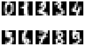

# target 데이터는?
digits_label = digits.target
print(digits_label.shape)
digits_label[:20]

(1797,)





array([0, 1, 2, 3, 4, 5, 6, 7, 8, 9, 0, 1, 2, 3, 4, 5, 6, 7, 8, 9])

총 1,797개의 데이터가 있고, 0부터 9까지의 숫자로 나타남.
바로 각 이미지 데이터가 어떤 숫자를 나타내는지를 담고 있는 데이터

붓꽃 문제와 같이,
각 이미지 데이터가 입력되었을 때
그 이미지가 숫자 몇을 나타내는
이미지인지를 맞추는 분류 모델을 학습

정확도의 함정을 확인하는 실험이기 때문에 약간의 장치를 넣어볼 것
->숫자 10개를 모두 분류하는 것이 아니라,
해당 이미지 데이터가 3인지 아닌지를 맞히는 문제로 변형해서 풀어보는 것

즉 입력된 데이터가 3이라면 3을,
3이 아닌 다른 숫자라면
0을 출력하도록 하는 모델을 생각

# target인 digits_label을 아래와 같이 살짝 변형
#  label인 digits_label에서 숫자가 3이라면 그대로 3을, 아니라면 0을 가지는 new_label
new_label = [3 if i == 3 else 0 for i in digits_label]
new_label[:20]

[0, 0, 0, 3, 0, 0, 0, 0, 0, 0, 0, 0, 0, 3, 0, 0, 0, 0, 0, 0]

digits_data와 new_label로 Decision Tree 모델을 학습, 정확도를 확인

train_test_split으로
학습 데이터와
테스트 데이터를 만든 후,
모델을 fit 시키고,
predict를 통해 예측 결과를 만든 후
accuracy_score를 이용해 정확도를 측정

# 참고 분꽃의 예

from sklearn.model_selection import train_test_split

X_train, X_test, y_train, y_test = train_test_split(iris_data,      
                                                    # iris_data는 문제지 :  feature
                                                    iris_label,     
                                                    # 맞춰야 할 정답값 : Label(3가지중)
                                                    test_size=0.2,  
                                                    # test dataset의 크기를 조절 : 전체의 20%만 테스트데이터로 사용
                                                    random_state=7) 
                                                    # train 데이터와 test 데이터를 분리(split)하는데 적용되는 랜덤성

print('X_train 개수: ', len(X_train),', X_test 개수: ', len(X_test))

X_train 개수:  120 , X_test 개수:  30

from sklearn.metrics import accuracy_score                    # 정확도 확인 모듈
from sklearn.model_selection import train_test_split          # 
from sklearn.tree import DecisionTreeClassifier               # Decision Tree Model

X_train, X_test, y_train, y_test = train_test_split(digits_data,     # digits_data 라는 문제지
                                                    new_label,       # 맞춰야할 정닶값
                                                    test_size=0.2,   # 전체의 20%만 테스트데이터로 사용
                                                    random_state=15) # train 데이터와 test 데이터를 분리(split)하는데 적용되는 랜덤성

decision_tree = DecisionTreeClassifier(random_state=15)       #디트리
decision_tree.fit(X_train, y_train)                           #디트리모델 Fit
y_pred = decision_tree.predict(X_test)                        #디트리모델 테스트로 예측

accuracy = accuracy_score(y_test, y_pred)                     #정확도 스코어 테스트와 예측값 비교
accuracy                                                      #값은

0.9388888888888889

모델이 전혀 학습하지 않고 정답을 모두 0으로만 선택해도 정확도가 90%가량이 나오게 된다는 것

# 길이는 y_pred와 같으면서 0으로만 이루어진 리스트를 fake_pred라는 변수로 저장해 보고, 
# 이 리스트와 실제 정답인 y_test간의 정확도를 확인.
fake_pred = [0] * len(y_pred)

accuracy = accuracy_score(y_test, fake_pred)
accuracy

0.925

정답을 모두 0으로만 선택해도 정확도가 90%가량이 나오게 된다는 것

이러한 문제는 불균형한 데이터, unbalanced 데이터에서 자주 발생할 수 있음

즉 정확도는 정답의 분포에 따라 모델의 성능을 잘 평가하지 못하는 척도가 될 수 있는 것

정답과 오답에도 종류가 있다!

오차 행렬(confusion matrix) : 정답과 오답을 구분하여 표현하는 방법

What is Confusion Matrix and Advanced Classification Metrics?

오차 행렬에서는 예측 결과를 네 가지로 구분

TN(True Negative), FP(False Positive), FN(False Negative), TP(True Positive)

오차 행렬에서 나타나는 성능 지표를 다섯 가지

Precision, Negative Predictive Value, Sensitivity, Specificity, Accuracy

TP, FN, FP, TN의 수치로 계산되는 성능 지표

정밀도(Precision)
- 높을수록 좋음
- TP / TP +FP
- 틀렸는데 맞다고 예측하면 안됨(Type 1 Error:FP:Precision)
재현율(Recall, Sensitivity)
- 높을수록 좋음
- 맞는데 틀렸다고 예측하면 안됨(type 2 Error:FN)
F1 스코어(f1 score)

Q17. 전체 메일함에서 스팸 메일을 거르는 모델에게는
Precision이 더 중요할까요, Recall이 더 중요할까요?
(스팸 메일을 positive, 정상 메일을 negative로 생각합니다)

예시답안

메일 처리 모델은 스팸 메일을 못 거르는 것은 괜찮지만,
정상 메일을 스팸 메일로 분류하는 것은 더 큰 문제이다.
즉 음성을 양성으로 판단하면 안 된다.
따라서 Precision이 더 중요하다.

실제(Actual Class)에서 뭐가 더 심각하냐. 문제가 크냐. 뭐가 중요하냐

실제 포지티브를 잘못 판단한게 중요 -> 포지티브가 중요 FN Recall
실제 네거티브를 잘못 판단한게 중요 -> 네거티브가 중요 FP Precision

==>>>정상이 중요

scikit-learn으로 이 지표들을 확인하는 방법

오차 행렬은 다음과 같이 sklearn.metrics 패키지 내의 confusion_matrix로 확인

from sklearn.metrics import confusion_matrix

confusion_matrix(y_test, y_pred)

array([[320,  13],
       [  9,  18]])

왼쪽 위부터 순서대로 TPTP, FNFN, FPFP, TNTN의 개수

#  모든 숫자를 0으로 예측한 fake_pred의 경우
confusion_matrix(y_test, fake_pred)

array([[333,   0],
       [ 27,   0]])

손글씨 결과의 Precision, Recall, F1 score는
sklearn.metrics의 classification_report를 활용.

from sklearn.metrics import classification_report

print(classification_report(y_test, y_pred))

              precision    recall  f1-score   support

           0       0.97      0.96      0.97       333
           3       0.58      0.67      0.62        27

    accuracy                           0.94       360
   macro avg       0.78      0.81      0.79       360
weighted avg       0.94      0.94      0.94       360

#  fake_pred의 경우

print(classification_report(y_test, fake_pred, zero_division=0))

              precision    recall  f1-score   support

           0       0.93      1.00      0.96       333
           3       0.00      0.00      0.00        27

    accuracy                           0.93       360
   macro avg       0.46      0.50      0.48       360
weighted avg       0.86      0.93      0.89       360

label이 불균형하게 분포되어있는 데이터를 다룰 때는 더 조심

정확도만으로 판단하지 말것.

데이터가 달라도 문제 없어요!

scikit-learn의 예제 데이터를 활용

데이터셋 소개 : 사이킷런 toy datasets

Toy Dataset 중 분류 문제에 적합한 데이터셋

load_digits : 손글씨 이미지 데이터
load_wine : 와인 데이터
load_breast_cancer : 유방암 데이터

1단계 : 데이터 확인하기

#  sklearn 라이브러리의 datasets 패키지 안 load_$$$$를 import 
#  $$$$ 데이터를 로딩
from sklearn.datasets import load_wine

print(wine.DESCR) # DESCR에는 데이터셋의 설명

.. _wine_dataset:

Wine recognition dataset
------------------------

**Data Set Characteristics:**

    :Number of Instances: 178 (50 in each of three classes)
    :Number of Attributes: 13 numeric, predictive attributes and the class
    :Attribute Information:
 		- Alcohol
 		- Malic acid
 		- Ash
		- Alcalinity of ash  
 		- Magnesium
		- Total phenols
 		- Flavanoids
 		- Nonflavanoid phenols
 		- Proanthocyanins
		- Color intensity
 		- Hue
 		- OD280/OD315 of diluted wines
 		- Proline

    - class:
            - class_0
            - class_1
            - class_2
		
    :Summary Statistics:
    
    ============================= ==== ===== ======= =====
                                   Min   Max   Mean     SD
    ============================= ==== ===== ======= =====
    Alcohol:                      11.0  14.8    13.0   0.8
    Malic Acid:                   0.74  5.80    2.34  1.12
    Ash:                          1.36  3.23    2.36  0.27
    Alcalinity of Ash:            10.6  30.0    19.5   3.3
    Magnesium:                    70.0 162.0    99.7  14.3
    Total Phenols:                0.98  3.88    2.29  0.63
    Flavanoids:                   0.34  5.08    2.03  1.00
    Nonflavanoid Phenols:         0.13  0.66    0.36  0.12
    Proanthocyanins:              0.41  3.58    1.59  0.57
    Colour Intensity:              1.3  13.0     5.1   2.3
    Hue:                          0.48  1.71    0.96  0.23
    OD280/OD315 of diluted wines: 1.27  4.00    2.61  0.71
    Proline:                       278  1680     746   315
    ============================= ==== ===== ======= =====

    :Missing Attribute Values: None
    :Class Distribution: class_0 (59), class_1 (71), class_2 (48)
    :Creator: R.A. Fisher
    :Donor: Michael Marshall (MARSHALL%PLU@io.arc.nasa.gov)
    :Date: July, 1988

This is a copy of UCI ML Wine recognition datasets.
https://archive.ics.uci.edu/ml/machine-learning-databases/wine/wine.data

The data is the results of a chemical analysis of wines grown in the same
region in Italy by three different cultivators. There are thirteen different
measurements taken for different constituents found in the three types of
wine.

Original Owners: 

Forina, M. et al, PARVUS - 
An Extendible Package for Data Exploration, Classification and Correlation. 
Institute of Pharmaceutical and Food Analysis and Technologies,
Via Brigata Salerno, 16147 Genoa, Italy.

Citation:

Lichman, M. (2013). UCI Machine Learning Repository
[https://archive.ics.uci.edu/ml]. Irvine, CA: University of California,
School of Information and Computer Science. 

.. topic:: References

  (1) S. Aeberhard, D. Coomans and O. de Vel, 
  Comparison of Classifiers in High Dimensional Settings, 
  Tech. Rep. no. 92-02, (1992), Dept. of Computer Science and Dept. of  
  Mathematics and Statistics, James Cook University of North Queensland. 
  (Also submitted to Technometrics). 

  The data was used with many others for comparing various 
  classifiers. The classes are separable, though only RDA 
  has achieved 100% correct classification. 
  (RDA : 100%, QDA 99.4%, LDA 98.9%, 1NN 96.1% (z-transformed data)) 
  (All results using the leave-one-out technique) 

  (2) S. Aeberhard, D. Coomans and O. de Vel, 
  "THE CLASSIFICATION PERFORMANCE OF RDA" 
  Tech. Rep. no. 92-01, (1992), Dept. of Computer Science and Dept. of 
  Mathematics and Statistics, James Cook University of North Queensland. 
  (Also submitted to Journal of Chemometrics).

#  sklearn 라이브러리의 datasets 패키지 안 load_$$$$를 import 
#  $$$$ 데이터를 로딩
from sklearn.datasets import load_breast_cancer

breast_cancer = load_breast_cancer()

print(breast_cancer.DESCR) # DESCR에는 데이터셋의 설명

.. _breast_cancer_dataset:

Breast cancer wisconsin (diagnostic) dataset
--------------------------------------------

**Data Set Characteristics:**

    :Number of Instances: 569

    :Number of Attributes: 30 numeric, predictive attributes and the class

    :Attribute Information:
        - radius (mean of distances from center to points on the perimeter)
        - texture (standard deviation of gray-scale values)
        - perimeter
        - area
        - smoothness (local variation in radius lengths)
        - compactness (perimeter^2 / area - 1.0)
        - concavity (severity of concave portions of the contour)
        - concave points (number of concave portions of the contour)
        - symmetry
        - fractal dimension ("coastline approximation" - 1)

        The mean, standard error, and "worst" or largest (mean of the three
        worst/largest values) of these features were computed for each image,
        resulting in 30 features.  For instance, field 0 is Mean Radius, field
        10 is Radius SE, field 20 is Worst Radius.

        - class:
                - WDBC-Malignant
                - WDBC-Benign

    :Summary Statistics:

    ===================================== ====== ======
                                           Min    Max
    ===================================== ====== ======
    radius (mean):                        6.981  28.11
    texture (mean):                       9.71   39.28
    perimeter (mean):                     43.79  188.5
    area (mean):                          143.5  2501.0
    smoothness (mean):                    0.053  0.163
    compactness (mean):                   0.019  0.345
    concavity (mean):                     0.0    0.427
    concave points (mean):                0.0    0.201
    symmetry (mean):                      0.106  0.304
    fractal dimension (mean):             0.05   0.097
    radius (standard error):              0.112  2.873
    texture (standard error):             0.36   4.885
    perimeter (standard error):           0.757  21.98
    area (standard error):                6.802  542.2
    smoothness (standard error):          0.002  0.031
    compactness (standard error):         0.002  0.135
    concavity (standard error):           0.0    0.396
    concave points (standard error):      0.0    0.053
    symmetry (standard error):            0.008  0.079
    fractal dimension (standard error):   0.001  0.03
    radius (worst):                       7.93   36.04
    texture (worst):                      12.02  49.54
    perimeter (worst):                    50.41  251.2
    area (worst):                         185.2  4254.0
    smoothness (worst):                   0.071  0.223
    compactness (worst):                  0.027  1.058
    concavity (worst):                    0.0    1.252
    concave points (worst):               0.0    0.291
    symmetry (worst):                     0.156  0.664
    fractal dimension (worst):            0.055  0.208
    ===================================== ====== ======

    :Missing Attribute Values: None

    :Class Distribution: 212 - Malignant, 357 - Benign

    :Creator:  Dr. William H. Wolberg, W. Nick Street, Olvi L. Mangasarian

    :Donor: Nick Street

    :Date: November, 1995

This is a copy of UCI ML Breast Cancer Wisconsin (Diagnostic) datasets.
https://goo.gl/U2Uwz2

Features are computed from a digitized image of a fine needle
aspirate (FNA) of a breast mass.  They describe
characteristics of the cell nuclei present in the image.

Separating plane described above was obtained using
Multisurface Method-Tree (MSM-T) [K. P. Bennett, "Decision Tree
Construction Via Linear Programming." Proceedings of the 4th
Midwest Artificial Intelligence and Cognitive Science Society,
pp. 97-101, 1992], a classification method which uses linear
programming to construct a decision tree.  Relevant features
were selected using an exhaustive search in the space of 1-4
features and 1-3 separating planes.

The actual linear program used to obtain the separating plane
in the 3-dimensional space is that described in:
[K. P. Bennett and O. L. Mangasarian: "Robust Linear
Programming Discrimination of Two Linearly Inseparable Sets",
Optimization Methods and Software 1, 1992, 23-34].

This database is also available through the UW CS ftp server:

ftp ftp.cs.wisc.edu
cd math-prog/cpo-dataset/machine-learn/WDBC/

.. topic:: References

   - W.N. Street, W.H. Wolberg and O.L. Mangasarian. Nuclear feature extraction 
     for breast tumor diagnosis. IS&T/SPIE 1993 International Symposium on 
     Electronic Imaging: Science and Technology, volume 1905, pages 861-870,
     San Jose, CA, 1993.
   - O.L. Mangasarian, W.N. Street and W.H. Wolberg. Breast cancer diagnosis and 
     prognosis via linear programming. Operations Research, 43(4), pages 570-577, 
     July-August 1995.
   - W.H. Wolberg, W.N. Street, and O.L. Mangasarian. Machine learning techniques
     to diagnose breast cancer from fine-needle aspirates. Cancer Letters 77 (1994) 
     163-171.

프로젝트

단계별 진행방법

필요한 모듈 Import

from sklearn.datasets import load_digits
from sklearn.model_selection import train_test_split
from sklearn.metrics import classification_report

데이터 확인하기

from sklearn.datasets import load_digits

print(digits.DESCR)

.. _digits_dataset:

Optical recognition of handwritten digits dataset
--------------------------------------------------

**Data Set Characteristics:**

    :Number of Instances: 1797
    :Number of Attributes: 64
    :Attribute Information: 8x8 image of integer pixels in the range 0..16.
    :Missing Attribute Values: None
    :Creator: E. Alpaydin (alpaydin '@' boun.edu.tr)
    :Date: July; 1998

This is a copy of the test set of the UCI ML hand-written digits datasets
https://archive.ics.uci.edu/ml/datasets/Optical+Recognition+of+Handwritten+Digits

The data set contains images of hand-written digits: 10 classes where
each class refers to a digit.

Preprocessing programs made available by NIST were used to extract
normalized bitmaps of handwritten digits from a preprinted form. From a
total of 43 people, 30 contributed to the training set and different 13
to the test set. 32x32 bitmaps are divided into nonoverlapping blocks of
4x4 and the number of on pixels are counted in each block. This generates
an input matrix of 8x8 where each element is an integer in the range
0..16. This reduces dimensionality and gives invariance to small
distortions.

For info on NIST preprocessing routines, see M. D. Garris, J. L. Blue, G.
T. Candela, D. L. Dimmick, J. Geist, P. J. Grother, S. A. Janet, and C.
L. Wilson, NIST Form-Based Handprint Recognition System, NISTIR 5469,
1994.

.. topic:: References

  - C. Kaynak (1995) Methods of Combining Multiple Classifiers and Their
    Applications to Handwritten Digit Recognition, MSc Thesis, Institute of
    Graduate Studies in Science and Engineering, Bogazici University.
  - E. Alpaydin, C. Kaynak (1998) Cascading Classifiers, Kybernetika.
  - Ken Tang and Ponnuthurai N. Suganthan and Xi Yao and A. Kai Qin.
    Linear dimensionalityreduction using relevance weighted LDA. School of
    Electrical and Electronic Engineering Nanyang Technological University.
    2005.
  - Claudio Gentile. A New Approximate Maximal Margin Classification
    Algorithm. NIPS. 2000.

데이터 준비

load_digits 메서드

digits = load_digits()

데이터 이해하기

Feature Data 지정하기
Label Data 지정하기
Target Names 출력해 보기
데이터 Describe 해 보기

train, test 데이터 분리

모델 학습과 테스트용 문제지와 정답지
X_train, X_test, y_train, y_test를 생성

다양한 모델로 학습

Decision Tree 사용해 보기
Random Forest 사용해 보기
SVM 사용해 보기
SGD Classifier 사용해 보기
Logistic Regression 사용해 보기

모델을 평가.

sklearn.metrics 에서 제공하는 평가지표

load_digits : 손글씨를 분류해 봅시다

load_wine : 와인을 분류해 봅시다

load_breast_cancer : 유방암 여부를 진단해 봅시다

프로젝트 제출

백건

마케팅을 위한 인공지능 설계와 스타트업 Log

이전 포스트

ᄂ 😄 [7 일차] : Flipped Units 36. 클래스 상속

다음 포스트

	sepal length (cm)	sepal width (cm)	petal length (cm)	petal width (cm)	label
0	5.1	3.5	1.4	0.2	0
1	4.9	3.0	1.4	0.2	0
2	4.7	3.2	1.3	0.2	0
3	4.6	3.1	1.5	0.2	0
4	5.0	3.6	1.4	0.2	0
...	...	...	...	...	...
145	6.7	3.0	5.2	2.3	2
146	6.3	2.5	5.0	1.9	2
147	6.5	3.0	5.2	2.0	2
148	6.2	3.4	5.4	2.3	2
149	5.9	3.0	5.1	1.8	2

	sepal length (cm)	sepal width (cm)	petal length (cm)	petal width (cm)	label
0	5.1	3.5	1.4	0.2	0
1	4.9	3.0	1.4	0.2	0
2	4.7	3.2	1.3	0.2	0
3	4.6	3.1	1.5	0.2	0
4	5.0	3.6	1.4	0.2	0
...	...	...	...	...	...
145	6.7	3.0	5.2	2.3	2
146	6.3	2.5	5.0	1.9	2
147	6.5	3.0	5.2	2.0	2
148	6.2	3.4	5.4	2.3	2
149	5.9	3.0	5.1	1.8	2