인공지능 스터디 7주차 - 비지도 학습(Unsupervised Learning)

1-1 군집화와 차원축소

• 군집화(클러스팅)
  라벨이 없는 예를 그룹화하는 것. 시장 세분화, 소셜 네트워크 분석, 검색결과 그룹화, 의료 영상, 이미지 세분화, 이상 감지 등에 사용된다. 클러스터링 후 각 클러스터에 클러스터 ID라는 번호가 할당된다.
  일반화 : 클러스터의 일부 예시에 특성 데이터가 누락된 경우 다른 예시에서 누락된 데이터를 추론할 수 있다.
  데이터 압축 : 데이터를 대체할 수 있는 특성으로 인해 특성 데이터가 간소화되고 스토리지가 절약된다.
  개인정보 보호 : 사용자를 클러스팅하고 데이터를 클러스터 ID와 연결하여 개인정보를 보존할수 있다.
  군집화 참고 링크
  
• 차원축소
  차원 축소는 주 변수 집합을 획득하여 임의 변수의 양을 줄이는 머신 러닝 혹은 통계 기법이다. 이 과정은 복잡한 문제의 모델링을 단순화하고, 중복을 제거하여 모델이 과적합이 될 가능성을 줄여준다. 차원 축소는 특징 선택과 특징 추출로 나뉘는데, 특징 선택은 필터링(filtering), 래핑(wrapping) 또는 포함(embedding)을 통해 다차원 데이터 셋으로부터 더 작은 하위집합이 모델을 표현하기 위해 선택된다. 특징 추출은 변수를 모델링하고 구성요소 분석을 위해 데이터 세트의 차원 수를 줄이는 것이다.
  <차원 축소 방법>
  • Factor Analysis
  • Low Variance Filter
  • High Correlation Filter
  • Backward Feature Elimination
  • Forward Feature Selection
  • Principal Component Analysis (PCA)
  • Linear Discriminant Analysis
  • Methods Based on Projections
  • t-Distributed Stochastic Neighbor Embedding (t-SNE)
  • UMAP
  • Independent Component Analysis
  • Missing Value Ratio
  • Random Forest
    차원축소 참고 사이트

---

1-2 K-Means

가장 고전적이고 직관적인 군집화 기법
1. 임의의 중심점 설정
임의의 장소에 사전에 설정해준 군집의 수만큼의 중심점을 배치해준다. 데이터를 잘 구분하기 위해서는 중심이 데이터들의 가운데에 있어야한다.
2. 평균의 중심으로 중심점 이동
각 데이터와 중심점 간의 거리를 계산하여 거리가 평균적으로 비슷할 때까지 중심점을 이동시킨다.
3. 중심점 확정 및 최종 군집화
위 방법을 계속 반복하여 더 이상 중심점이 움직이지 않는 순간이 오도록 한다.

*K-means알고리즘은 데이터간의 거리로 군집화를 진행하기 떄문에 멀리 떨어져있는 데이터에 관해서는 취약하다.

#군집화용 데이터를 생성하고 산점도를 그려본다.
import pandas as pd
import numpy as np
import matplotlib.pyplot as plt

from sklearn.datasets import make_blobs

X, y = make_blobs(n_samples=500, 
               n_features=2, 
               centers=3,
               cluster_std=2, 
               random_state=42)
df = pd.DataFrame(data=X, columns = ["x1", "x2"])
df['label'] = y

target_list = np.unique(y)
color_lst = ['r', 'g', 'b']

for target, color in zip(target_list, color_lst) :
   target_cl = df[df['label']==target]
   plt.scatter(x=target_cl['x1'], y = target_cl['x2'], edgecolor = 'k', color = color)
   
plt.show()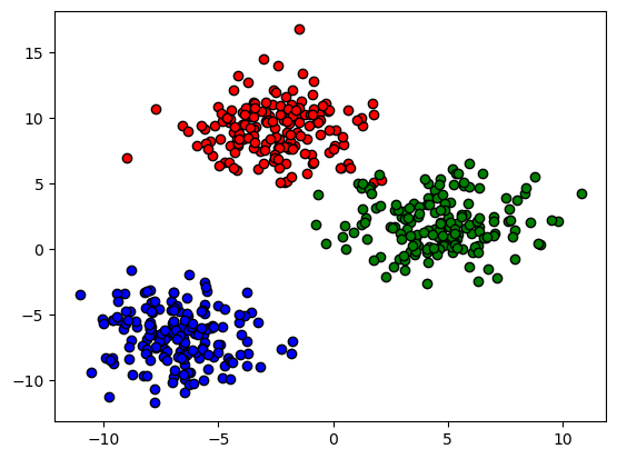

#군집화 진행
import pandas as pd
import numpy as np

from sklearn.cluster import KMeans

kmeans = KMeans(n_clusters=3, random_state = 42)       #KMeans알고리즘 실행 코드
kmeans.fit(X)
cluster_labels = kmeans.labels_

df['clusters'] = cluster_labels

centers = kmeans.cluster_centers_
unique_labels = np.unique(cluster_labels)
markers=['o', 's', '^', 'P','D','H','x']

for label in unique_labels:
    label_cluster = df[df['clusters']==label]
    center_x_y = centers[label]
    plt.scatter(x=label_cluster['x1'], y=label_cluster['x2'], edgecolor='k', 
                marker=markers[label] )

    plt.scatter(x=center_x_y[0], y=center_x_y[1], s=200, color='white',
                alpha=0.9, edgecolor='k', marker=markers[label])
    plt.scatter(x=center_x_y[0], y=center_x_y[1], s=70, color='k', edgecolor='k', 
                marker='$%d$' % label)

plt.show()

print()
print("👀실제 값과 군집 비교👀")
print(df.groupby('label')['clusters'].value_counts())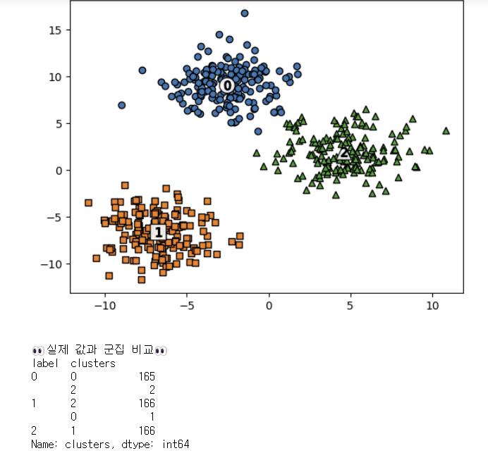

참고사이트

---

1-3 실루엣 계수

군집이 잘 형성되었는지 확인하는 지표
실루엣 계수 : 군집 내의 데이터끼리 얼마나 잘 뭉쳐있는지, 다른 군집의 데이터와는 얼마나 멀리 떨어져 있는지 측정하는 지표. -1~1 사이의 값을 가진다. (-1일수록 좋지 않음)

from sklearn.metrics import silhouette_score, silhouette_samples

## 각 데이터별 실루엣 점수
samples = silhouette_samples(X.data, df['clusters'])  #silhouette_samples
df['silhouette'] = samples

## 전체 실루엣 점수
score = silhouette_score(X.data, df['clusters'])    #silhouette_score
print(f"🚀전체 실루엣 점수🚀\n{score:.2f}\n")
print("📃군집별 평균 실루엣 점수📃")
print(df.groupby('clusters')['silhouette'].mean())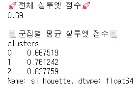

참고사이트

<KMeans 외에 다른 군집화 기법>
DBSCAN(밀도 기반 클러스터링): 밀도가 높은 부분을 클러스터링 하는 방식
GMM(가우시안 혼합 모델): Gaussian 분포가 여러 개 혼합된 클러스터링 알고리즘
계층적 군집화 : 여러개의 군집 중에서 가장 유사도가 높은 군집 두개를 선택하여 하나로 합치는 것

---

2-1 차원축소

데이터를 묘사하는 Feature가 너무 많으면 혼란을 초래하기 때문에 효율적으로 줄여야할 필요가 있다.
1. Feature Selection : 말그대로 필요한 Feature만 선택
2. Feature Extraction : 기존의 Feature를 살짝 변형하여 압축. 대표기법 PCA(공분산, 고유벡터, 고유값 개념 필요)

#PCA 기법 사용
import pandas as pd
import numpy as np
from sklearn.datasets import *
from sklearn.preprocessing import StandardScaler
from sklearn.decomposition import PCA

X, y = load_iris(return_X_y=True, as_frame=True)
normal_dataset = pd.concat([X, y], axis=1)

ss = StandardScaler()
scaled_X = ss.fit_transform(X)

pca = PCA(n_components=2)        #PCA 코드
pca_features = pca.fit_transform(scaled_X)   #fit_transform
pca_col_lst = [f"pca_{i}" for i in range(1, pca_features.shape[1]+1)]
pca_dataset = pd.DataFrame(pca_features, columns=pca_col_lst)
pca_dataset = pd.concat([pca_dataset, y], axis=1)

print("🚩압축된 각 축이 전체 변수를 얼마나 설명하는지🚩")
print(pca.explained_variance_ratio_, f"-> 전체 설명률 : {sum(pca.explained_variance_ratio_)*100:.2f}%")

pca_dataset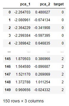

---

2-2 차원축소 전과 후 성능 비교 해보기

압축된 변수들로 학습시킨 모델의 성능 차이 비교(분류모델은 RandomForest)

from sklearn.metrics import classification_report
from sklearn.model_selection import train_test_split
from sklearn.ensemble import RandomForestClassifier

## normal dataset 
X_train, X_val, y_train, y_val = train_test_split(X, y, test_size=0.2, random_state=42)
rf_clf = RandomForestClassifier(random_state = 42)
rf_clf.fit(X_train, y_train)
preds= rf_clf.predict(X_val)
print("🤖일반 데이터셋 성능🤖")
print(classification_report(y_val, preds))

## PCA datset
pca_X_tr, pca_X_val, pca_y_tr, pca_y_val = train_test_split(pca_features, y, test_size=0.2, random_state=42)
rf_clf = RandomForestClassifier(random_state = 42)
rf_clf.fit(pca_X_tr, pca_y_tr)
pca_preds= rf_clf.predict(pca_X_val)
print("🤖PCA 데이터셋 성능🤖")
print(classification_report(pca_y_val, pca_preds))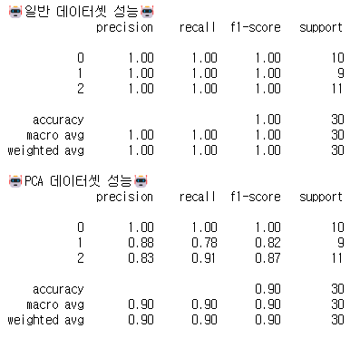

---

2-3 차원축소 변수의 의미 해석

Loading : 원본 변수가 각 PCA축에 기여하는 정도

loadings = pd.DataFrame(pca.components_.T, columns=pca_col_lst,index=X.columns)
loadings.sort_values(by="pca_1", ascending=False)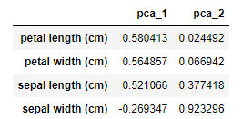

보통 절대값이 클 수록, 해당 변수가 축을 만들 때 많이 기여했다고 해석한다.
petal length이 pca_1에 많이 기여했고, sepal width가 pca_2에 많은 기여를 했다.