이 포스트는 Causal Inference and Discovery in Python책의 Chapter9의 내용을 바탕으로 작성하였습니다.

Implementing Matching & IPW

그럼 실제로, Matching과 IPW를 이용해서 효과를 추정해보도록 하겠습니다.

Load Data

해당 데이터는 ‘took a course’, ‘age’, ‘earnings’ 정보가 담겨있습니다.

이 데이터로 ‘강좌 수강 여부’가 ‘소득’에 미치는 영향을 추정해보겠습니다.

earnings_data = pd.read_csv(r'./data/ml_earnings.csv')

단순하게 효과를 추정하면, 어떻게 나올까요?

# Compute naive estimate 
treatment_avg = earnings_data.query('took_a_course==1')['earnings'].mean()
cntrl_avg = earnings_data.query('took_a_course==0')['earnings'].mean()

treatment_avg - cntrl_avg

# 6695.57

실제 효과가 10,000니까, 약 33%의 MAPE를 갖습니다. 굉장히 크네요!

그럼 이제 Matching/IPW를 통해 보다 정확한 추정을 해보겠습니다.

Define the graph

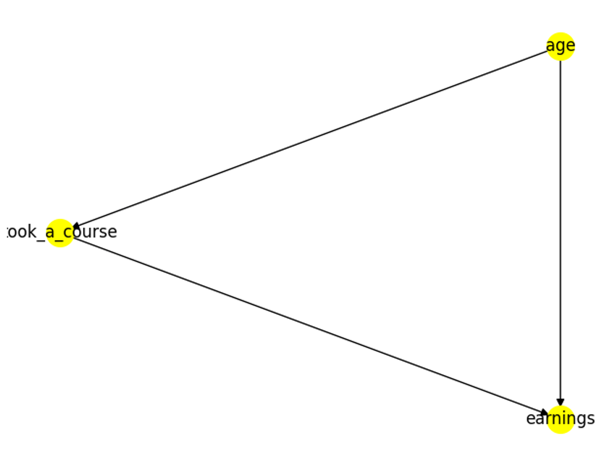
model을 만들기 위해 causal graph를 정의합니다.

# Define GMLGraph function
def GMLGraph(nodes, edges):
    # Generate the GML graph
    gml_string = 'graph [directed 1\n'
    
    for node in nodes:
        gml_string += f'\tnode [id "{node}" label "{node}"]\n'
    
    for edge in edges:
        gml_string += f'\tedge [source "{edge[0]}" target "{edge[1]}"]\n'
    
    gml_string += ']'
    return gml_string

# Construct the graph (the graph is constant for all interations)
nodes = ['took_a_course','earnings','age']
edges = [
    ('took_a_course','earnings'),
    ('age','took_a_course'),
    ('age','earnings')
]

gml_graph = GMLGraph(nodes,edges)

# Instantiate the CausalModel
model = CausalModel(
    data=earnings_data,
    treatment='took_a_course',
    outcome='earnings',
    graph=gml_graph
)

Get the estimand

confounder가 있는 인과구조이기 때문에, ‘backdoor’ estimand를 써야겠죠?

실제로, 사용할 estimand를 확인해봐도 동일한 결과를 결과를 얻을 수 있습니다.

(frontdoor estimand는 ‘chain’ 형태일 때, iv는 ‘iv’가 존재할 때 사용할 수 있습니다.)

# Get the estimand
estimand = model.identify_effect()

print(estimand)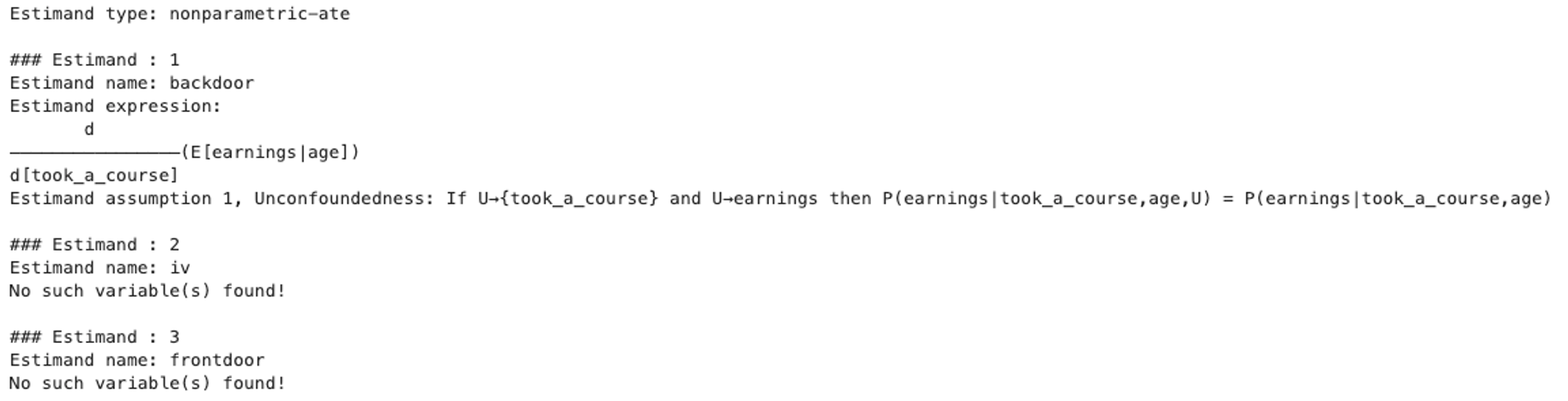

Estimate the effect

이제 Matching/IPW를 이용해서 효과를 추정하고 두 결과를 비교해보겠습니다.

1) Matching

우선 Matching 방법입니다.

# Get estimate (Matching)
estimate = model.estimate_effect(
    identified_estimand=estimand,
    method_name='backdoor.distance_matching',
    target_units='ate',
    method_params={'distance_metric':'minkowski','p':2})

estimate.value

여기선 비슷한 unit을 매칭하기 위해, p=2인 Minkowski distance를 사용했습니다.

p=2이기 때문에 Minkowski distance는 Euclidean distance와 동일합니다.

참고) Minkowski distance

$D(X,Y)=(\sum_{i=1}^n{|x_{i}-y_{i}|^p})^{\frac{1}{p}}$

여기선, 변수가 하나이기 때문에, standardization/normalization 할 필요없습니다.

하지만, 변수가 여러개라면 scale에 따라 distance에 영향을 주는 정도가 다르기 때문에 standardization/normalization이 필요할 수 있습니다.

해당 전처리를 하지 않는 것이 더 정확하다는 주장도 있기 때문에, 이는 개인의 선택입니다.

위 방법으로 추정하면 효과가 ‘10333.75’로 나옵니다!

MAPE가 3.34%로 naive estimator에 비해 훨씬 줄어들었습니다.

이 결과를 ‘random_common_cause’ 방법을 이용해서 검증해보겠습니다.

refutation = model.refute_estimate(
    estimand=estimand,
    estimate=estimate,
    method_name='random_common_cause')

random_common_cause는 random한 값으로 이루어진 confounder를 인과 그래프에 추가한 후 결과가 동일한지 확인하는 방법입니다.

random한 값이기 때문에 결과가 동일해야 하고, 만약 결과가 달라진다면 해당 추정치는 unobserved confounder에 의해 robust하지 않다는 것을 의미합니다.

print(refutation)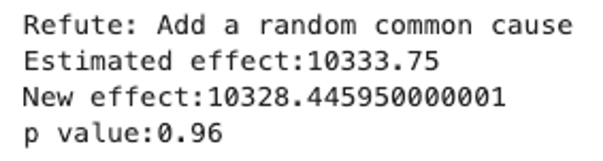

결과가 조금 달라지긴 했지만, 귀무가설(두 값은 동일하다)에 대한 p-value가 0.96이기 때문에 통계적으로 유의하지 않습니다.

2) IPW

IPW estimator 중 ‘backdoor.propensity_score_weighting’ 방법을 사용해보겠습니다.

해당 방법은 weighted least squares(wls) 를 사용하여 효과를 추정합니다.

우선, control variable인 age로 earnings을 추정함으로써 propensity score를 구하고,

이 propensity score를 가중치 하는 wls를 통해 ate를 계산합니다.

estimate_ipw = model.estimate_effect(
    identified_estimand=estimand,
    method_name='backdoor.propensity_score_weighting',
    target_units='ate'
)

print(estimate_ipw.value)
# 10313.57

IPW로 계산한 효과는 10313.57로 Matching에 비해 MATE가 다소 줄어들었습니다(3.34% → 3.14%).

보통 Matching이 IPW보다 정확도가 높다고 알려져 있긴 하지만, 이는 task마다 다를 수 있습니다.

Key Points

Matching과 IPW를 이용해서 실제 효과를 추정해봤습니다.

DoWhy 패키지를 이용하면 두 방법 모두 쉽게 사용할 수 있습니다.

task에 따라 적절한 방법이 다를 수 있기 때문에, 어떤 방법이 적절할지 고민해보고 task에 맞는 방법을 사용하면 좋을 것 같습니다.