시각화: CAM (Class Activation Mapping) + GAP (Global Average Pooling)

설명가능한 인공지능(Explainable AI, XAI)은 판단에 대한 이유를 사람이 이해할 수 있는 방식으로 제시하는 인공지능이다. (from 위키피디아)

사람이 직관적으로 이해하지 못하는 모델을 블랙박스 모델이라고 하는데, 이런 모델은 현업에서 의사결정권자들을 설득하지 못하는 등의 문제가 존재한다. (ex 성능은 좋은데 이유를 모르겠어!)

예를 들어 선형회귀와 같은 기법은 어느 정도 통계적 지식이 있는 사람들은 쉽게 이해할 수 있는 반면 복잡한 (흔히 딥러닝이라 불리는) 모델은 직관적으로 이해하기 힘들다. 결국 여러개의 logit 반복

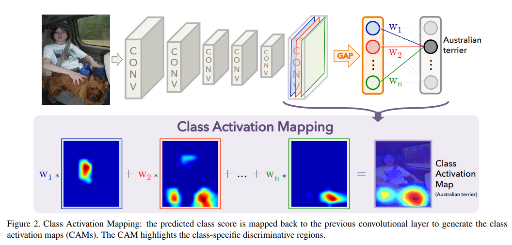
CAM (Class Activation Mapping)은 설명가능한 인공지능 기술 중 하나로, 데이터의 어느 부분이 모델의 의사결정에 큰 영향을 미쳤는지 시각화하는 기법이다. (마지막 feature extraction map을 기준으로)

아래 그림과 같이 모델이 australian terrier가 위치한 지역을 결정하는데, 이미지의 어느 부분이 큰 영향을 미쳤는지 시각화해주는 방법이다.

1. 라이브러리

import numpy as np
from matplotlib import pyplot as plt
import cv2

import torch
import torchvision
import torchvision.transforms as transforms
from torch.utils.data import DataLoader
import torch.nn as nn
import torch.optim as optim

device = torch.device("cuda:0" if torch.cuda.is_available() else "cpu")

2. 데이터 및 모델 생성 (CAM 적용을 위한)

transform = transforms.Compose([transforms.Resize(128), transforms.ToTensor(), transforms.Normalize((0.5, 0.5, 0.5), (0.5, 0.5, 0.5))])
trainset = torchvision.datasets.STL10(root='./data', split='train', download=True, transform=transform) # 96x96
trainloader = torch.utils.data.DataLoader(trainset, batch_size=40, shuffle=True)

model = torchvision.models.resnet18(pretrained=True)
num_ftrs = model.fc.in_features # fc의 입력 노드 수를 산출한다. 512개
model.fc = nn.Linear(num_ftrs, 10) # fc를 nn.Linear(num_ftrs, 10)로 대체한다.
model = model.to(device)

3. 모델 학습 (CAM 적용을 위한)

criterion = nn.CrossEntropyLoss()
optimizer = optim.Adam(model.parameters(), lr=1e-4, weight_decay=1e-2)

for epoch in range(20):

    running_loss = 0.0
    for data in trainloader:
        
        inputs, labels = data[0].to(device), data[1].to(device)
          
        optimizer.zero_grad()
        outputs = model(inputs)
        loss = criterion(outputs, labels)
        loss.backward()
        optimizer.step()

        running_loss += loss.item()

    cost = running_loss / len(trainloader)        
    print('[%d] loss: %.3f' %(epoch + 1, cost))  

torch.save(model.state_dict(), './models/stl10_resnet18.pth')      

print('Finished Training')

4. 학습결과 확인

correct = 0
total = 0
with torch.no_grad():
    model.eval()
    for data in trainloader:
        images, labels = data[0].to(device), data[1].to(device)
        outputs = model(images)
        _, predicted = torch.max(outputs.data, 1)
        total += labels.size(0)
        correct += (predicted == labels).sum().item()

print('Accuracy of the network on the train images: %d %%' % (100 * correct / total))

# result
Accuracy of the network on the train images: 95 %

모델의 마지막 구조 확인 (resnet 18)

(~이전 생략)

  (layer4): Sequential(
    (0): BasicBlock(
      (conv1): Conv2d(256, 512, kernel_size=(3, 3), stride=(2, 2), padding=(1, 1), bias=False)
      (bn1): BatchNorm2d(512, eps=1e-05, momentum=0.1, affine=True, track_running_stats=True)
      (relu): ReLU(inplace=True)
      (conv2): Conv2d(512, 512, kernel_size=(3, 3), stride=(1, 1), padding=(1, 1), bias=False)
      (bn2): BatchNorm2d(512, eps=1e-05, momentum=0.1, affine=True, track_running_stats=True)
      (downsample): Sequential(
        (0): Conv2d(256, 512, kernel_size=(1, 1), stride=(2, 2), bias=False)
        (1): BatchNorm2d(512, eps=1e-05, momentum=0.1, affine=True, track_running_stats=True)
      )
    )
    (1): BasicBlock(
      (conv1): Conv2d(512, 512, kernel_size=(3, 3), stride=(1, 1), padding=(1, 1), bias=False)
      (bn1): BatchNorm2d(512, eps=1e-05, momentum=0.1, affine=True, track_running_stats=True)
      (relu): ReLU(inplace=True)
      (conv2): Conv2d(512, 512, kernel_size=(3, 3), stride=(1, 1), padding=(1, 1), bias=False)
      (bn2): BatchNorm2d(512, eps=1e-05, momentum=0.1, affine=True, track_running_stats=True)
    )
  )
  (avgpool): AdaptiveAvgPool2d(output_size=(1, 1))
  (fc): Linear(in_features=512, out_features=10, bias=True)
)

 print(model.layer4[1]) # 결국 이 부분 시각화 하는것 
 
 #result
 BasicBlock(
  (conv1): Conv2d(512, 512, kernel_size=(3, 3), stride=(1, 1), padding=(1, 1), bias=False)
  (bn1): BatchNorm2d(512, eps=1e-05, momentum=0.1, affine=True, track_running_stats=True)
  (relu): ReLU(inplace=True)
  (conv2): Conv2d(512, 512, kernel_size=(3, 3), stride=(1, 1), padding=(1, 1), bias=False)
  (bn2): BatchNorm2d(512, eps=1e-05, momentum=0.1, affine=True, track_running_stats=True)
)

(이후 생략~)

5. CAM 모델 구축

# Visualize feature maps
activation = {} # 빈 dictionary

def get_activation(name):
    def hook(model, input, output):
        activation[name] = output.detach()
    return hook

def cam(model, trainset, img_sample, img_size):
    model.eval()
    with torch.no_grad(): # requires_grad 비활성화

        model.layer4[1].bn2.register_forward_hook(get_activation('final')) 
        # feature extraction의 마지막 feature map 구하기 (layer4[1])
        
        data, label = trainset[img_sample] # 이미지 한 장과 라벨 불러오기
        data.unsqueeze_(0) # 4차원 3차원 [피쳐수 ,너비, 높이] -> [1,피쳐수 ,너비, 높이]
        
        output = model(data.to(device))
        _, prediction = torch.max(output, 1)
        
        act = activation['final'].squeeze() # 4차원 [1,피쳐수 ,너비, 높이] -> 3차원 [피쳐수 ,너비, 높이]
        w = model.fc.weight # classifer의 가중치 불러오기
        
        for idx in range(act.size(0)): # CAM 연산 (결국 for loop으로 모든 가중치 합하는 것!!)
            if idx == 0:
                tmp = act[idx] * w[prediction.item()][idx] # 각 label에 해당하는 가중치
            else:
                tmp += act[idx] * w[prediction.item()][idx]

        # 모든 이미지 팍셀값을 0~255로 스케일하기 
        normalized_cam = tmp.cpu().numpy()
        normalized_cam = (normalized_cam - np.min(normalized_cam)) / (np.max(normalized_cam) - np.min(normalized_cam))
        original_img = np.uint8((data[0][0] / 2 + 0.5) * 255) 

        # 원본 이미지 사이즈로 리사이즈
        cam_img = cv2.resize(np.uint8(normalized_cam * 255), dsize=(img_size, img_size)) 
        
    return cam_img, original_img
    
def plot_cam(model, trainset, img_size, start):
    end = start + 20 # 결과 20장 나오게
    fig, axs = plt.subplots(2, (end - start + 1) // 2, figsize=(20, 5))
    fig.subplots_adjust(hspace=.01, wspace=.01)
    axs = axs.ravel()

    for i in range(start, end):
        cam_img, original_img = cam(model, trainset, i, img_size) # cam 이미지 나오는 부분 (오리지널 이미지 , CAM 이미지)

        axs[i - start].imshow(original_img, cmap='gray') # 오리지널은 gray
        axs[i - start].imshow(cam_img, cmap='jet', alpha=.5) # 빨파, alpha는 밝기
        axs[i - start].axis('off')

    plt.show()
    fig.savefig('cam.png')   
 
plot_cam(model, trainset, 128, 10)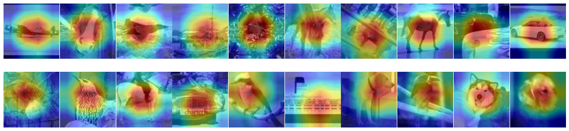

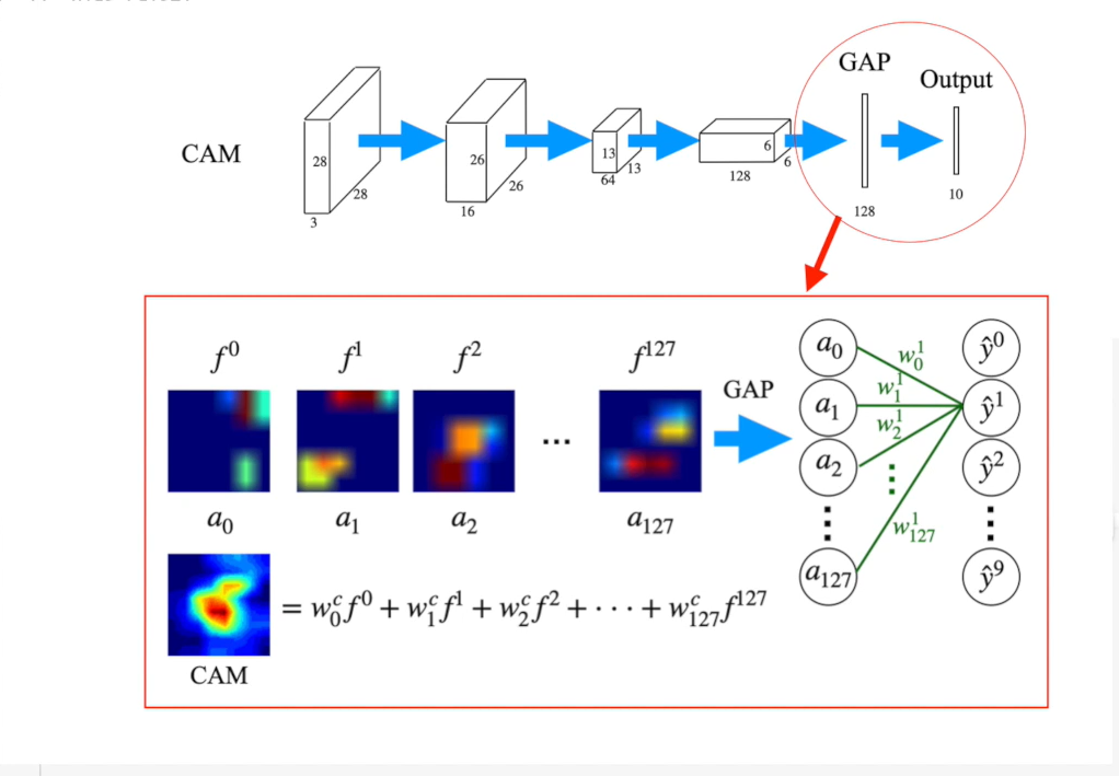
* CAM은 결국 feature extraction에 weight를 곱한 값의 합임!

GAP은 Max pooling 보다 더 급격하게 차원을 줄이는 방법인데, 주로 feature를 1차원 벡터로 만들기 위해 사용된다.

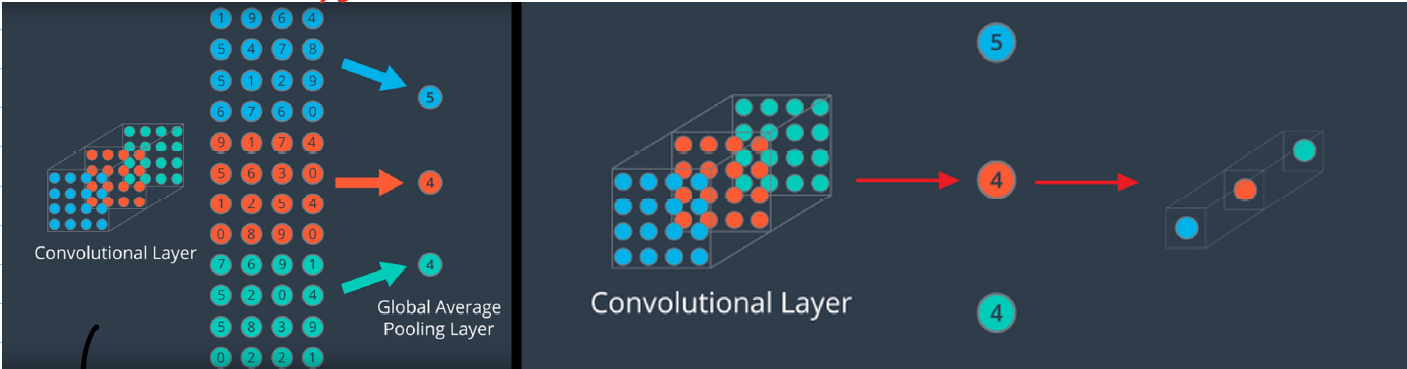
보통의 vision 모델은 CNN + FC (fully connected) Layer 구조. GAP은 classifier인 FC layer 를 없애기 위해 사용됨. FC layer는 마지막 feature와 matrix 곱을 하여 feature 전체를 연산의 대상으로 삼아서 결과를 출력함. (즉, feature가 이미지 전체를 함축하고 있다고 가정)

하지만, FC layer를 classifier로 사용하면 파라미터 수가 증가 + feature 전체를 matrix 연산하기 때문에 위치에 대한 정보가 사라지게 됨.

하지만 GAP은 어떤 크기의 feature라도 같은 채널의 값들을 하나의 평균(average)으로 대체하기 때문에 벡터의 형식으로 나옴. 즉, 어떤 사이지의 입력이 들어와도 상관이 없고 공간에 대한 정보를 유지하기 때문에 학습에 유리한 편!

대충 이런 느낌: (H, W, C) -> GAP -> (1, 1, C)