시각화: t-SNE (t-Stochastic Neighbor Embedding)

t-SNE는 PCA 더불어 대중적(?)으로 사용되는 차원 축소 기법이다. 현업에서 사용되는 데이터는 수 ~ 수백 차원으로 이루어진 경우가 많은데, 이런 경우 데이터의 분포 확인이나 시각화 진행에 어려움이 있다. 이런 경우 보통 2~3차원으로 데이터를 축소하는데 이를 차원 축소라 말한다.

1. 라이브러리

from sklearn.manifold import TSNE # sklearn 사용하면 easy !! 
import numpy as np
from matplotlib import pyplot as plt

import torch
import torchvision
import torchvision.transforms as transforms
from torch.utils.data import DataLoader
import torch.nn as nn

device = torch.device("cuda:0" if torch.cuda.is_available() else "cpu")

2. 데이터 불러오기 (CIFAR 10)

transform = transforms.Compose([transforms.ToTensor(), transforms.Normalize((0.5, 0.5, 0.5), (0.5, 0.5, 0.5))])
testset = torchvision.datasets.CIFAR10(root='./data', train=False, download=True, transform=transform)
testloader = torch.utils.data.DataLoader(testset, batch_size=16)

3. 시각화에 사용할 모델 불러오기

Fully connected 부분을 indentitiy로 바꿔주는 class (512개의 average pooling 값이 나옴)

class Identity(nn.Module):
    def __init__(self):
        super(Identity, self).__init__()

    def forward(self, x):
        return x

model = torchvision.models.resnet18(pretrained=False)
num_ftrs = model.fc.in_features # fc의 입력 노드 수를 산출한다. 512개
model.fc = nn.Linear(num_ftrs, 10) # fc를 nn.Linear(num_ftrs, 10)로 대체, CIFAR10,,
model = model.to(device)

# classifier 들어가기 직전에 값을 뽑아낼 것임
# (avgpool): AdaptiveAvgPool2d(output_size=(1, 1))
print(model)

# result
# (이전 생략) 마지막 부분 fully connected
    (1): BasicBlock(
      (conv1): Conv2d(512, 512, kernel_size=(3, 3), stride=(1, 1), padding=(1, 1), bias=False)
      (bn1): BatchNorm2d(512, eps=1e-05, momentum=0.1, affine=True, track_running_stats=True)
      (relu): ReLU(inplace=True)
      (conv2): Conv2d(512, 512, kernel_size=(3, 3), stride=(1, 1), padding=(1, 1), bias=False)
      (bn2): BatchNorm2d(512, eps=1e-05, momentum=0.1, affine=True, track_running_stats=True)
    )
  )
  (avgpool): AdaptiveAvgPool2d(output_size=(1, 1))
  (fc): Linear(in_features=512, out_features=10, bias=True)
)

classifier 들어가기 직전의 값을 뽑아내면

model.load_state_dict(torch.load('./models/cifar10_resnet18.pth'))
model.fc = Identity() # resnet18의 fc 부분을 위에서 만든 indentity class로 대체! 

# result
    (1): BasicBlock(
      (conv1): Conv2d(512, 512, kernel_size=(3, 3), stride=(1, 1), padding=(1, 1), bias=False)
      (bn1): BatchNorm2d(512, eps=1e-05, momentum=0.1, affine=True, track_running_stats=True)
      (relu): ReLU(inplace=True)
      (conv2): Conv2d(512, 512, kernel_size=(3, 3), stride=(1, 1), padding=(1, 1), bias=False)
      (bn2): BatchNorm2d(512, eps=1e-05, momentum=0.1, affine=True, track_running_stats=True)
    )
  )
  (avgpool): AdaptiveAvgPool2d(output_size=(1, 1))
  (fc): Identity()
)
# fc: indentity로 바뀜! 

4. t-SNE 모델로 evlauation 결과 확인 (각 class별 분포를 알아보자)

actual = []
deep_features = []

model.eval() # resnet18
with torch.no_grad():
    for data in testloader:
        images, labels = data[0].to(device), data[1].to(device)
        features = model(images) # 512 차원

        deep_features += features.cpu().numpy().tolist()
        actual += labels.cpu().numpy().tolist()

tsne = TSNE(n_components=2, random_state=0) # 사실 easy 함 sklearn 사용하니..
cluster = np.array(tsne.fit_transform(np.array(deep_features)))
actual = np.array(actual)

plt.figure(figsize=(10, 10))
cifar = ['plane', 'car', 'bird', 'cat', 'deer', 'dog', 'frog', 'horse', 'ship', 'truck']
for i, label in zip(range(10), cifar):
    idx = np.where(actual == i)
    plt.scatter(cluster[idx, 0], cluster[idx, 1], marker='.', label=label)

plt.legend()
plt.show()

5. 시각화 결과

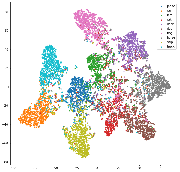
자동차랑 트럭이랑 비슷하고,,, bird랑 airplane 비슷하게 나옴